Part 1: Frequency Domain
Overview
Digital images are typically interpreted through the spatial domain. That is, the intensity of the various pixels in an image matrix is information represented in the spatial domain. But the spatial domain of an image can be processed and transformed to the frequency domain. The frequency domain reveals patterns behind the distribution of pixel values in the image. By identifying these patterns, we can isolate and utilize them to enhance, filter and blend these images.
Part 1.1: Warm-Up
Unsharp Masking Technique
By taking the second derivative of the spatial domain, we can isolate the high frequency information of the picture. Another way to achieve this is by applying a Gaussian filter (designed to strip the original image of high frequency information) to the orignal image and subtract that filtered image from original image. The result is an image consisting of the outlines of the subjects in the picture. The unsharp masking technique takes this high frequency information and adds it back to the original image to sharpen and boost its defining features.
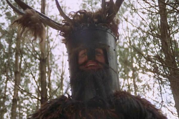 Before sharpening.
|
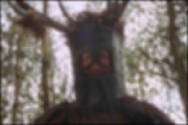
 After sharpening. The man's face is still blurry (maybe his features blend into each other) but the tree branches are much more distinct.
|
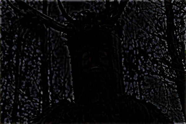
 Gaussian blurred image that is subtracted from the original image to create the image to the right.
|
 The high frequency information added to the original image to create the sharpened image.
|
 I might not be a robot but that captcha is still a little hard to read.
|
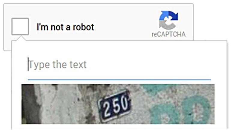 That's better!
|
Part 1.2: Hybrid Images
Frequency Analysis
We lose the high frequency information of objects the farther they are from us. The general shape of the object, the low frequency information, is preserved. Hybrid images take advantage of our eyes to contain two different images visible clearly at certain distances.
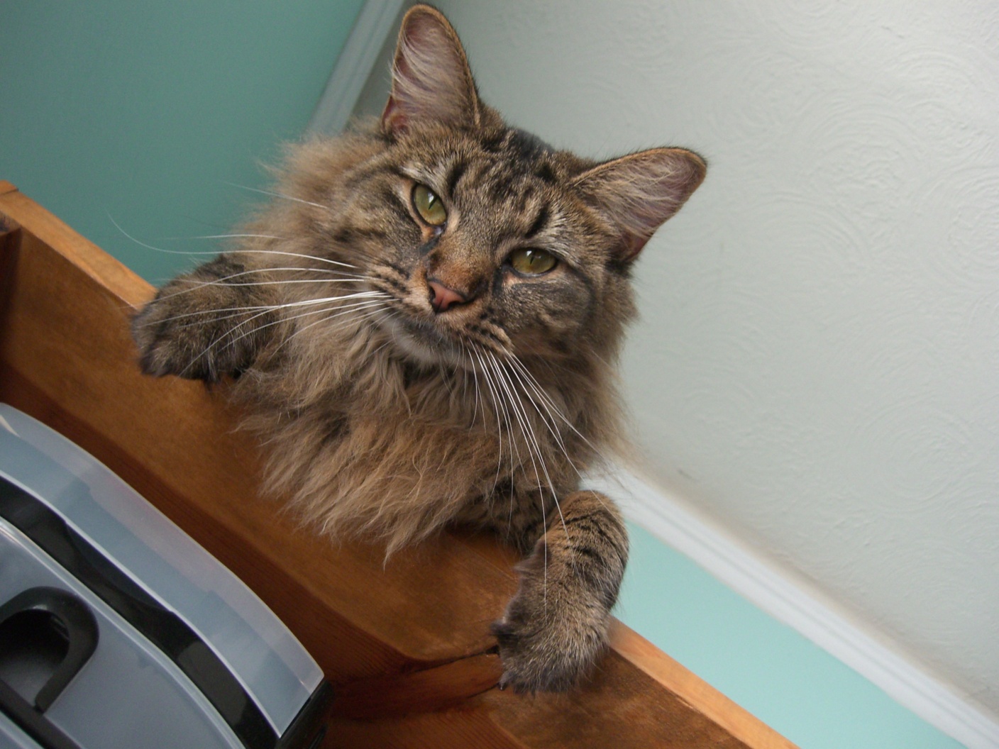 Unaltered photo of Nutmeg. To be processed so that only high freq info remains.
|
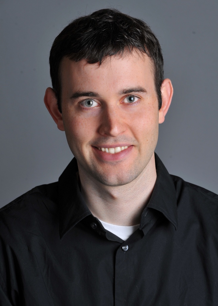 Unaltered photo of Derek. To be processed so that only low freq info remains.
|
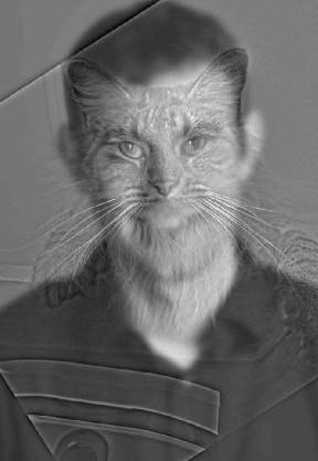 Hybrid image of Nutmeg and Derek. Derekmeg.
|
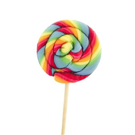 Unaltered photo of a lollipop. To be processed so that only high freq info remains.
|
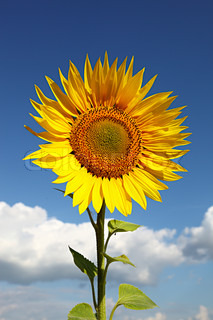 Unaltered photo of a sunflower. To be processed so that only low freq info remains.
|
 Hybrid image of a sunflower and lollipop. This combination was a failure because the detail on the sunflower was too high frequency. The blurred sunflower obscured the detail of the lollipop too much for this hybrid pairing to work.
|
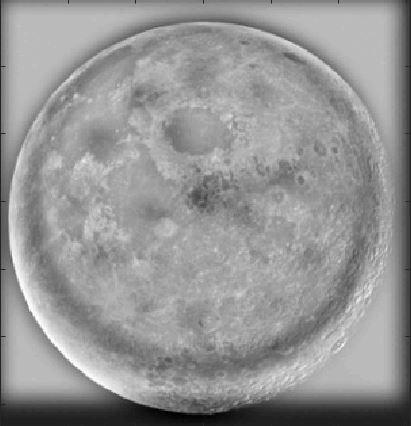
A hybrid image is a combination of two pictures, one with high frequency data and one with low frequency data. We get the low frequency data by convolving the photo with a Gaussian filter. I used one of size [30 30] with a sigma value of 7. We get the high frequency data by subtracting a Gaussian filtered image from the original image. The filter used here was of size [60 60] with a sigma value of 7. This is the same process used to get the "detail" for the unsharp masking technique. The photos below show the log magnitude of the Fourier transforms of the two input images as they are filtered and combined.
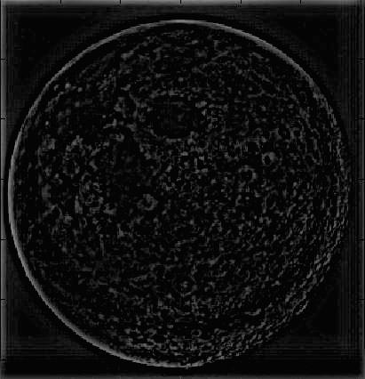
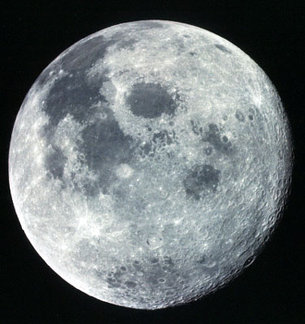 Unaltered photo of the moon.
|
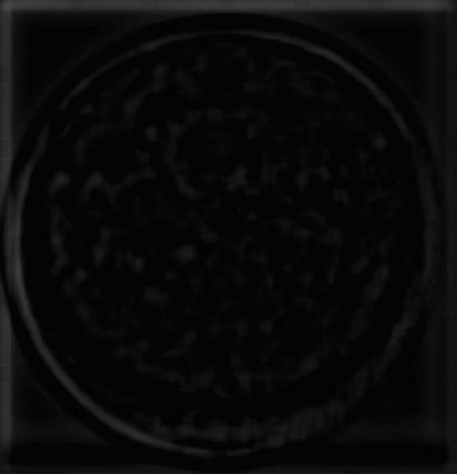
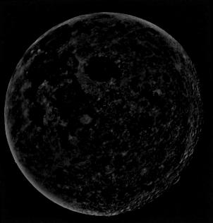 Band-pass filtered photo of the moon.
|
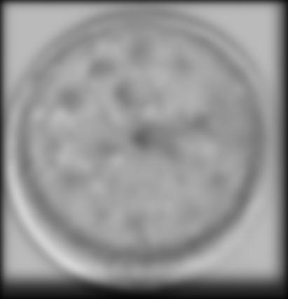
 Unaltered photo of an ornate clock.
|
 Fourier transform of the unprocessed photo of the moon.
|
 Fourier transform of the band-pass filtered moon.
|
 Fourier transform of the unprocessed photo of an ornate clock.
|
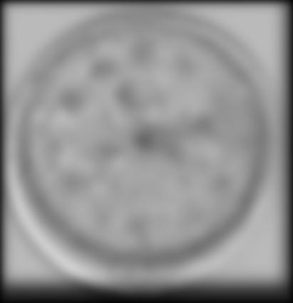
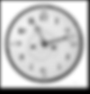 Low-pass filtered photo of an orate clock.
|
 Hybrid image of the moon and clock. This one requires some squinting!
|
 Fourier transform of the low-pass filtered clock.
|
 Fourier transform of the hybrid image.
|
Bells & Whistles: Colorized Hybrid Images
Using color salvaged the illusion of some of the hybrid images for me. Color in the "sunpop" hybrid image makes the lollipop jump just enough from the background to be visible. I tried different combinations of coloring the lollipop/sunflower as seen below. The first row of images has the sunflower being the low frequency component. The second row has the lollipop being the low frequency component. When color is added to both images, the presence of both images is clear from any distance. Color adds some low frequency detail across the spectrum, even for the high frequency components. If only the low frequency element is colored, it seems to imbue those colors into the high frequency image embedded in it. If only the high frequency element is colored, the low frequency only seems to serve as a backdrop. The color in the high frequency neutralizes the ability to block it from a distance.
 Both images are colored.
|
 Only the sunflower is colored.
|
 Only the lollipop is colored.
|
 Both images are colored.
|
 Only the lollipop is colored.
|
 Only the sunflower is colored.
|
The computation time does increase by a noticeable factor; it took about 5 seconds for Derekmeg to finish processing.
 Colorized version of the hybrid image Derekmeg.
|
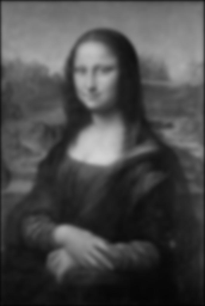
Part 1.3: Gaussian and Laplacian Stacks
What is a Gaussian stack? What is a Laplacian stack?
A Gaussian stack is a series of images that is recursively convolved with a Gaussian filter. The result is a series of images that get progressively blurrier. A Laplacian stack captures the high frequency information that is lost with each convolution in the Gaussian Stack. Each level of a Laplacian stack is the result of an image in an earlier level (less blurry) in the Gaussian stack subtracted by an image from the next step (more blurry) in the Gaussian stack. The last step in a Laplacian stack is the last step of the Gaussian stack. This allows the Laplacian stack to reconstruct the original image by summing all steps together.
Multiple Resolution Pictures
 Mona Lisa Laplacian Stack, Step 1. 3 steps total.
|
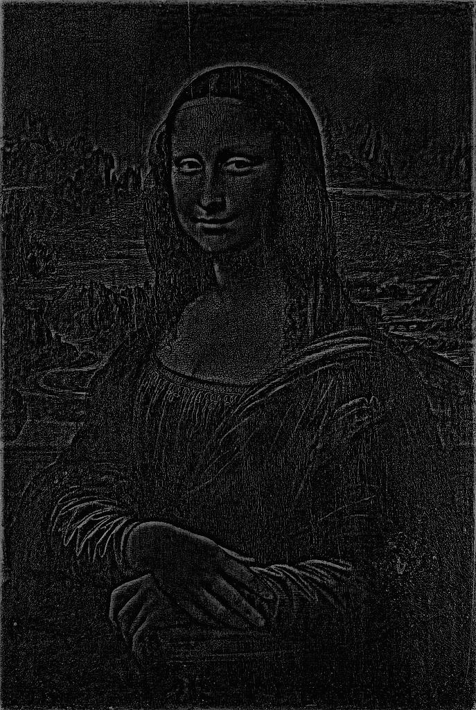
 Mona Lisa Laplacian Stack, Step 2
|
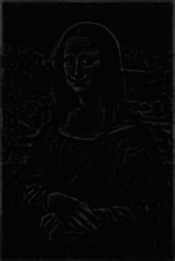
 Mona Lisa Laplacian Stack, Step 3
|
 Mona Lisa Laplacian Stack, Step 1
|
 Mona Lisa Laplacian Stack, Step 2
|
 Mona Lisa Laplacian Stack, Step 3
|
Steps of a Gaussian and Laplacian Stack on a Hybrid Image
 Moonclock Gaussian Stack, Step 1. This is the original image.
|
 Moonclock Gaussian Stack, Step 2
|
 Moonclock Gaussian Stack, Step 3
|
 Moonclock Gaussian Stack, Step 4
|
 Moonclock Gaussian Stack, Step 5
|
 Moonclock Laplacian Stack, Step 1
|
 Moonclock Laplacian Stack, Step 2
|
 Moonclock Laplacian Stack, Step 3
|
 Moonclock Laplacian Stack, Step 4
|
 Moonclock Laplacian Stack, Step 5. This step is the corresponding Gaussian step.
|
Part 1.4: Multiresolution Blending
Image Splines for Smooth Blending
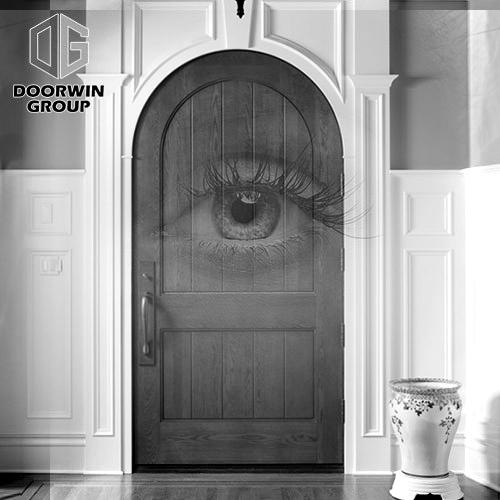
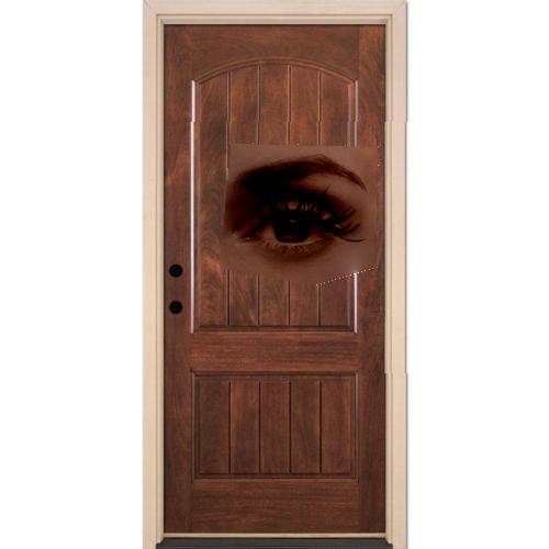
Multiresolution blending joins two images together at multiple frequency levels. Laplacian stacks formed from the two original images are joined together with the Gaussian stack formed from the alpha mask that demarcates the seam. At the lowest (blurriest) levels, the boundaries of the seam are generous. The seam at the highest level is very fine. The summation of these joined layers results in a convincing blend.
Multiple Resolution Pictures
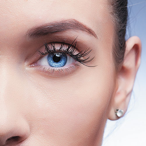 EYE PICTURE
|
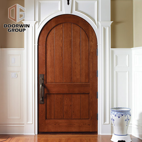 DOOR PICTURE
|
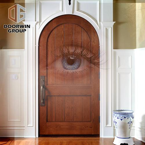 Watching door. The mask for this image was a little too broad but the eye is nicely blended in the door
|
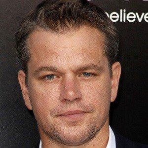
 MATT DAMON
|
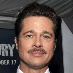
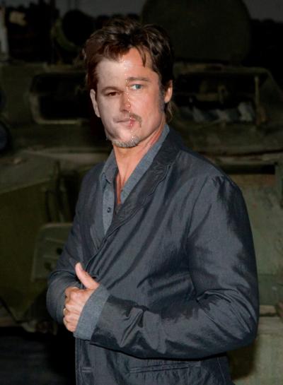
 BRAD PITT
|
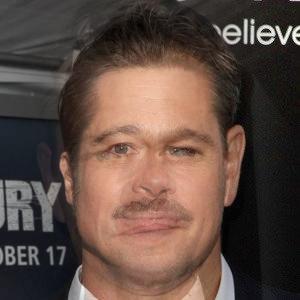 Brad Damon or Matt Pitt? Either way, this blend was a failure because their facial features did not align. The seam between their heads is convincing enough though.
|
 Mask used for watching door.
|
 Mask used for Matt/Brad and Oraple.
|
The contrast was boosted on shots of the Laplacian mask to make them more visible. You can see as the steps get deeper, the seam between the two is less fine.
Combination of various band-pass filtered images to the orange-apple mosiac
 Orapple, left-masked Laplacian step 1
|
 Orapple, right-masked Laplacian step 1
|
 Orapple, blended step 1
|
 Orapple, left-masked Laplacian step 3
|
 Orapple, right-masked Laplacian step 3
|
 Orapple, blended step 3
|
 Orapple, left-masked Laplacian step 7
|
 Orapple, right-masked Laplacian step 7
|
 Orapple, blended step 7
|
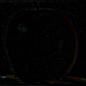
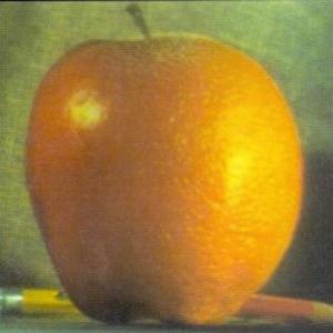 Final blend of Orapple. This is the combined sum of all 10 levels of the masked Laplacian stacks.
|
Bells & Whistles: Colorized Multiresolution Blending
Adding color makes discontinuites in the seam more apparent. The subjects themselves remain convincingly integrated but the increased realism makes your eyes question the image more. This is in the best case, where the two images being merged have a similar color profile. When the colors contrast, the area where the mask ends at the lowest resolutions is detectable.
Grayscale vs. Color
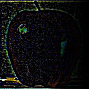
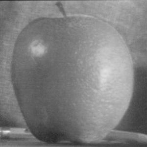 Orapple, in grayscale.
|
Orapple, colorized.
|
 Eyedoor, in grayscale.
|
Eyedoor, colorized.
|
Part 2: Gradient Domain Fusion
Overview
The gradient domain of an image can be found by taking its derivative. This gives us the general layout/pattern of the pixel intensities of an image. Just as our eyes filter out far away information by seeing only the low frequencies, our eyes also rely on gradients to easily categorize and distinguish information. If an image has a smooth gradient profile, we tend to perceive it as a cohesive image. If say we cropped a picture of a deer and pasted it into a desert scene, the deer would stick out like a sore thumb. The image it was ripped from had a gradient profile of its own, and now that we've inserted it into another image, it doesn't fit. Even if you could create a perfect mask to include only the deer, its presence would still be suspicious. Enter gradient domain fusion. By sampling from the gradient domain of the area immediately surrounding the deer, we can reconstruct the image to better match the gradient profile of the area. Even though we cannot replicate the lighting and other environmental conditions, the blended image will better appear to "belong" in the image.
Part 2.1: Toy Problem
What is the Toy Problem?
Given the gradient domain of an image and a single pixel, is it possible to reconstruct the original image? Yes, because that information allows us to construct a least squares problem in the form (Av - b)^2. v is a vector containing all the pixel information of the reconstructed image. We don't have that so we can solve for it by working with A and b. b is a vector containing the x and y gradient information of the original image, along with any other extra constraints. A is a matrix containing all the constraints that, when evaluated with v, should result in values close to or equal to b. When measuring differences in pixel intensities, my reconstructed image had an error of 0+1.9216e-06i.
 Original photo.
|
 Reconstructed photo.
|
Part 2.2: Poisson Blending
Poisson and Image Blending
Poisson blending uses the same format of reconstructing an image by formulating it as a least squares problem. This time, we are attempting to embed an image (the source) into a larger background image (the target). Unlike the toy problem, we have the gradient information from two images. So we can do more than simply reconstruct our source image in the background image. On the borders between our source image and target image, we have the opportunity to sample the gradient information from the target image. By adding this information to the b vector of our least square problem (Av = b), we can have least squares "spread" this information throughout the pixel intensities it determines when solving for v. If the two input images are similar in color, the result is a well-integrated image that can fool the human eye.
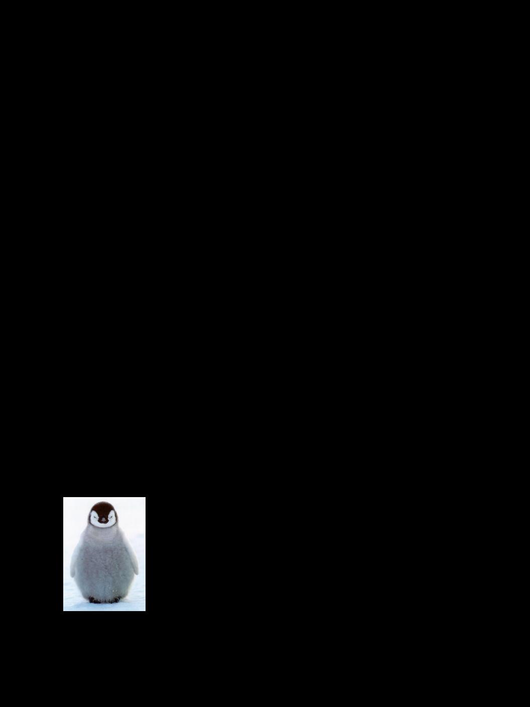
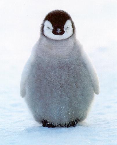 Source image of penguin.
|
 Target image of snowy mountain.
|
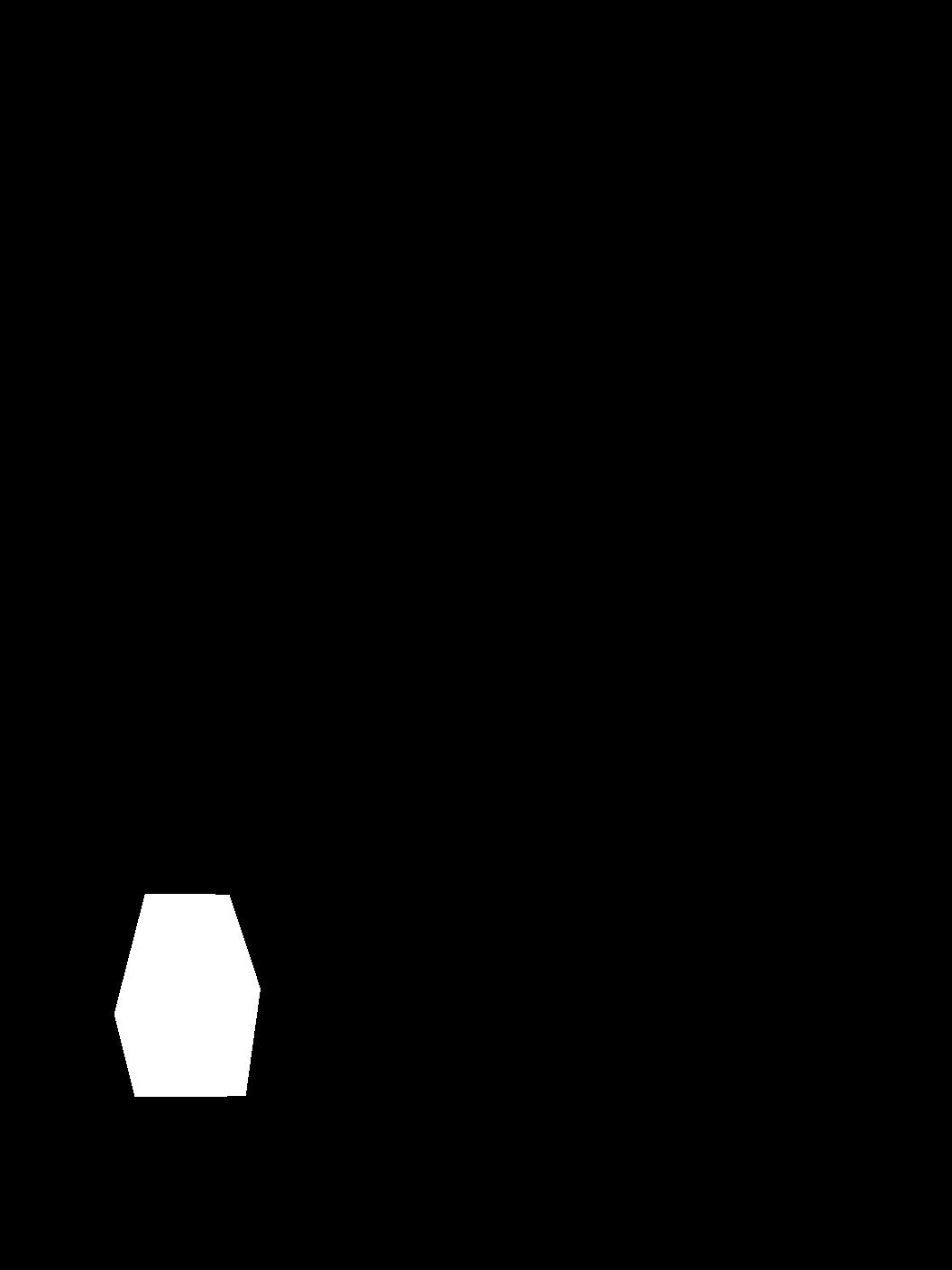 Mask of the target image. White is where penguin is to be placed.
|
 Penguin will be placed in this area of the target image.
|
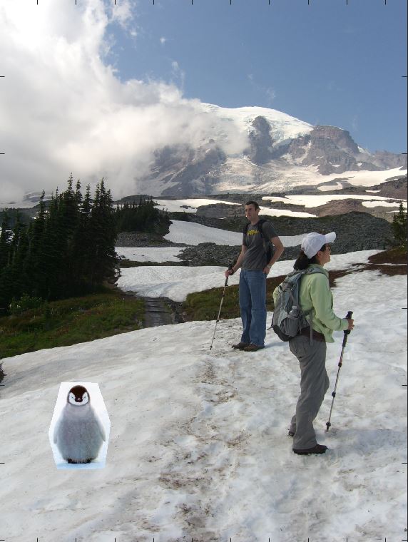 Penguin overlaid directly on image. Before poisson blending.
|
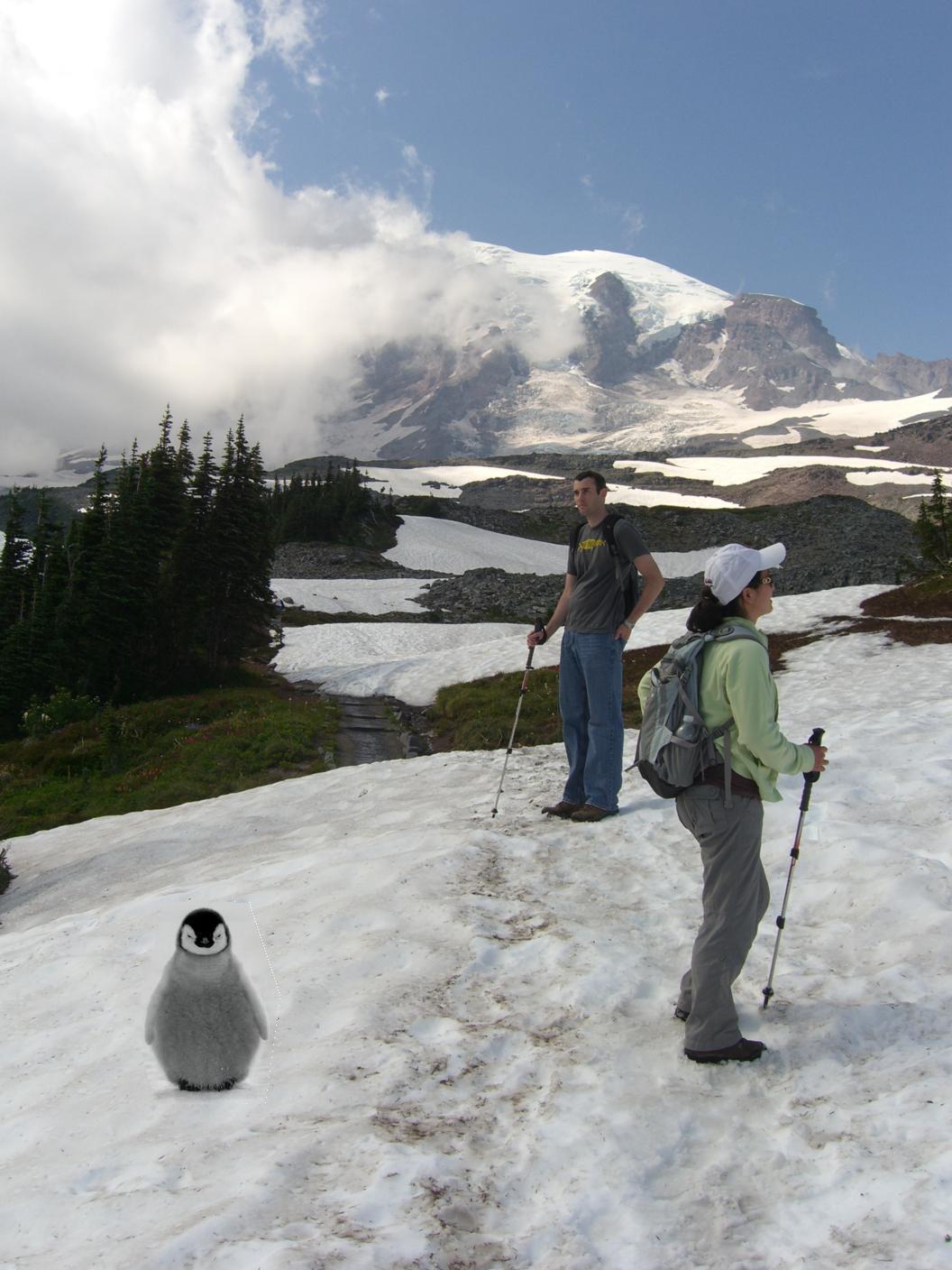 After poisson blending. The penguin and its surrounding have been changed to better fit into the image.
|
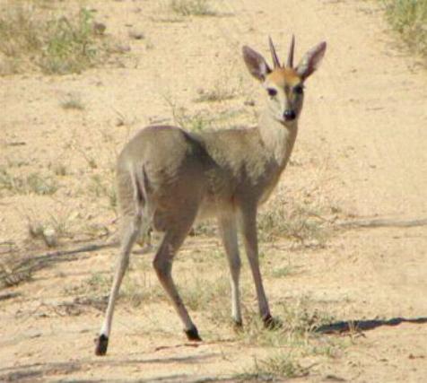 Source image of deer.
|
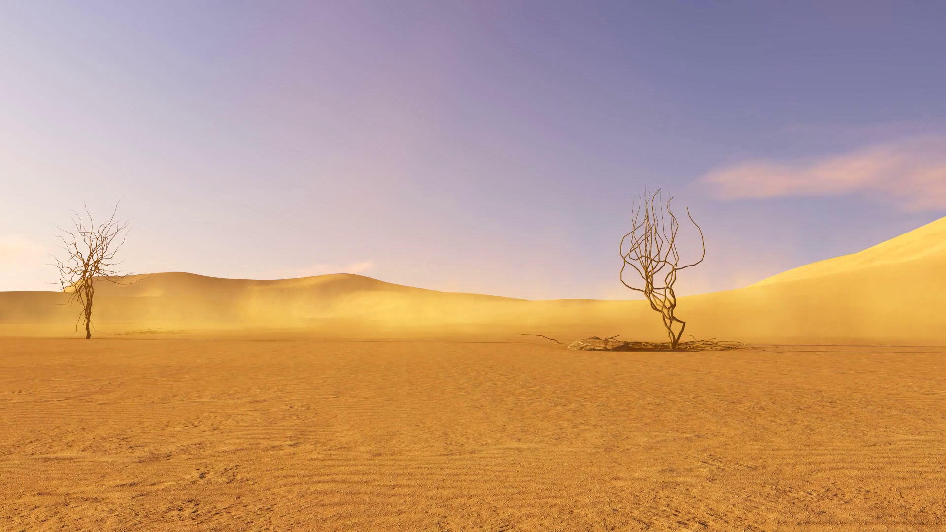 Target image of desert.
|
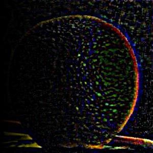
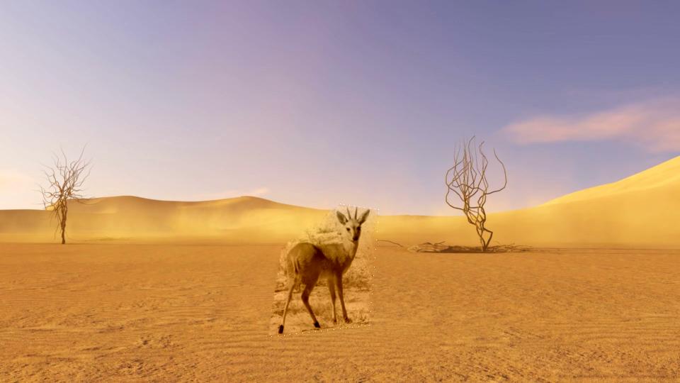 Deersert v1.0. This iteration was a failure because the foliage surrounding the original deer image is too high frequency to fit properly into the scene. The sand is also high detail, making for an even starker contrast.
|
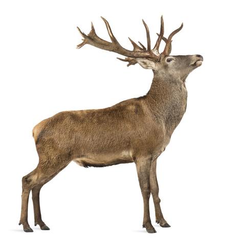 Source image of deer 2.0.
|
Target image of desert.
|
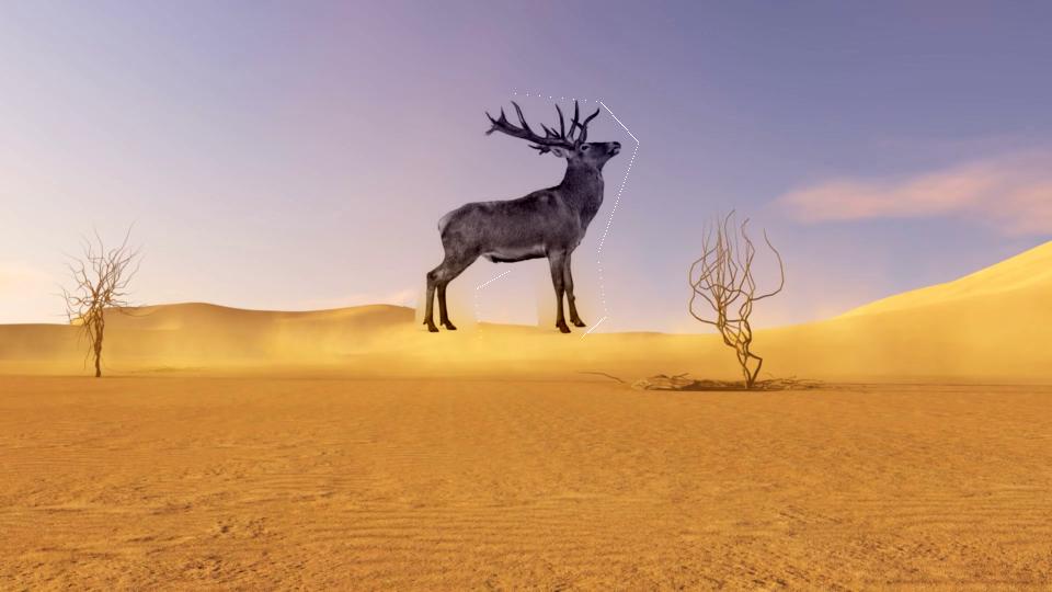 Deersert v2.0. The size may be offputting but the colors of the image blend pretty well into the top of the dunes and the sky (except for the white borders: more on that below).
|
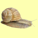 Source image of snail.
|
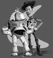
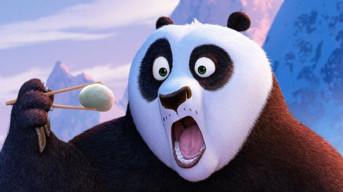 Target image of Po.
|
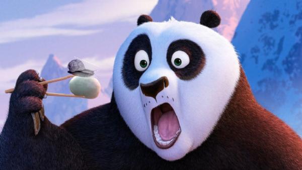 Po wasn't quick enough...
|
I had a LOT of trouble with this section. The border bug must have been a result of the border conditions setting the boundary pixel to a value of 1, but I couldn't find it after (many) hours of searching. The issues that plagued me consisted of MATLAB limitations (can't index into a 2D matrix with two boolean masks as indices) and image_alignment (had to search and align the image) with the mask. The MATLAB limitations prevented me from using objmask to build my A matrix efficiently; I had to loop through entire A matrix to remove gradient constraints for pixels that were outside the cropped mask.
Multiresolution vs. Poisson
Which approach works best for these images? Why? When do you think that one approach would be more appropriate than another?
Both approaches work to fool the eye, multiresolution with multiple frequency layers and Poisson with smooth gradient levels. Color in general is harmful to the reception of both of these approaches. I'd say the best approach for merging two objects together is multiresolution blending. It does not entirely strip an image of its color; instead it takes in the details of the other image it merges with as a complement to its own color. However, creating masks for this type of blending requires much more precision if wanting to insert it into a specific place. This is an area that poisson excels at. Although Poisson blending does not do well to preserve the color of the image ,that works in its favor when placing an object into a similarly colored environment. In the end, I'd say multiresolution does well for "merging" images and Poission does well for "embedding" images.
|
Matt Pitt with multiresolution blending.
|
 Brad Damon with Poisson blending.
|
 LAP RESULT
|
POISSON RESULT
|