Project 3: Fun with Frequencies and Gradients

Raymond Chu - cs194-26-aak

Part 1: Frequency Domain

Part 1-1: Warmup

The images are sharpened by subtracting a Gaussian filtered image from the original and then adding that difference back to the original image to accentuate edges.

→

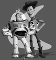
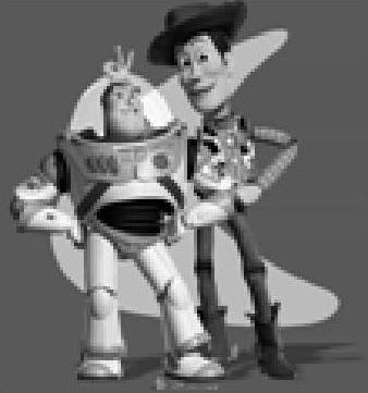
Part 1-2: Hybrid Images

We create hybrid images by taking high frequencies from one image and adding the low frequencies of another image. The low frequency image is obtained using a low-pass filter (Gaussian filter) and the high frequency image is obtained with a high-pass filter (Laplacian filter).

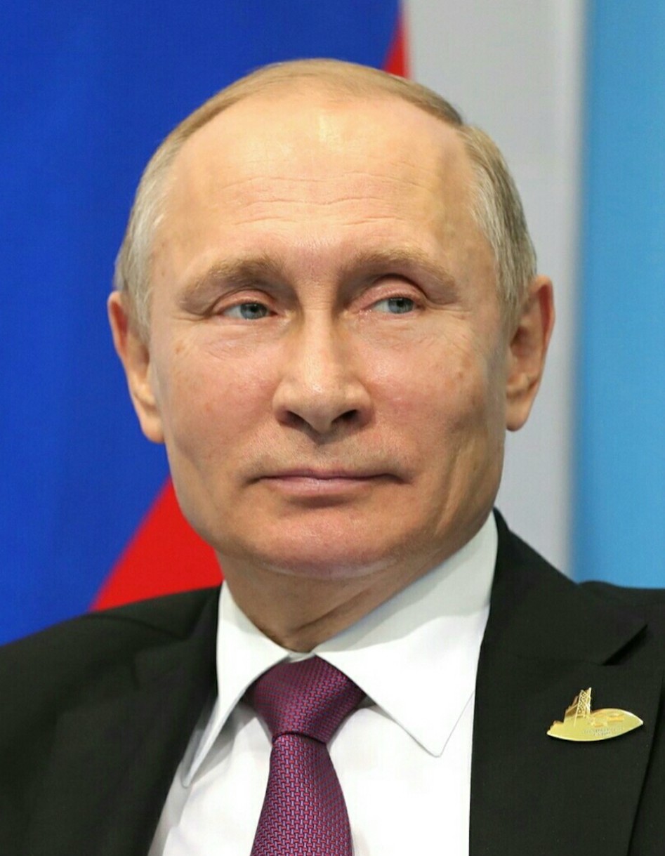
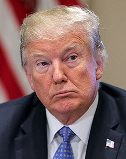
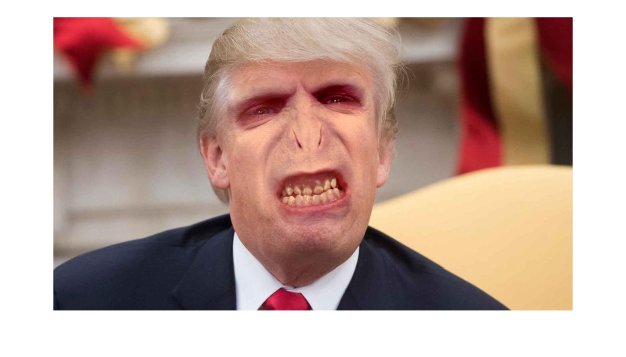
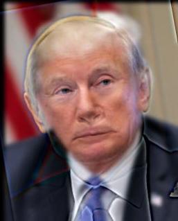
Original Putin	Original Trump	Final Blended Putin and Trump
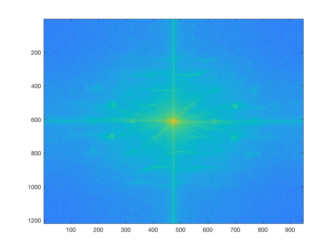
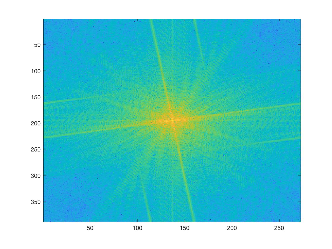
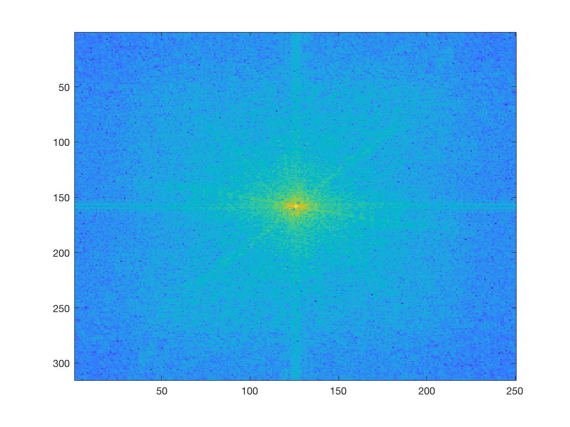
Original Putin FFT	Original Trump FFT
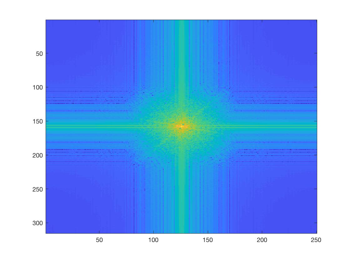
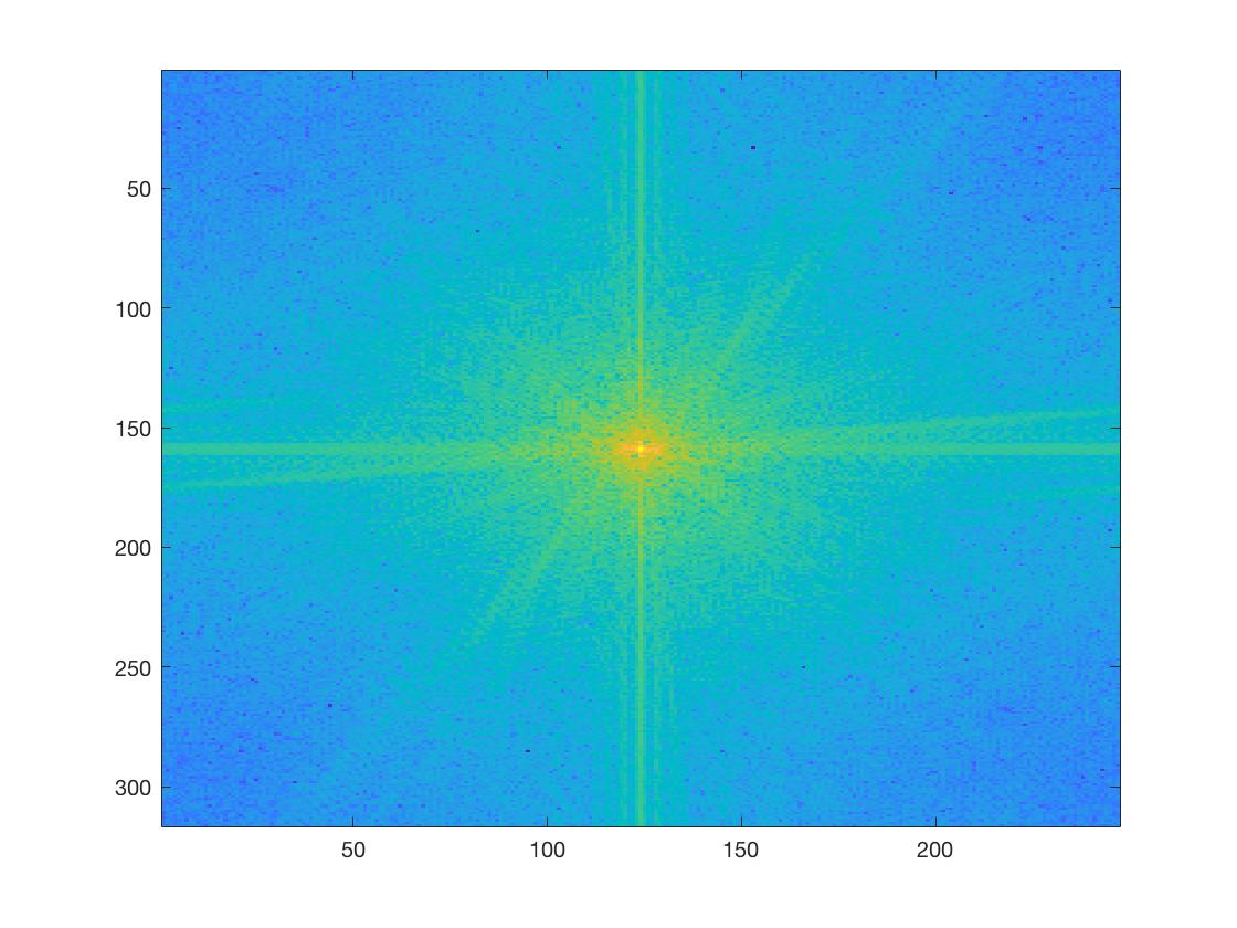
Filtered Putin FFT	Filtered Trump FFT	Filtered Putin/Trump Hybrid FFT

Final Hybrid Images

Putin and Trump

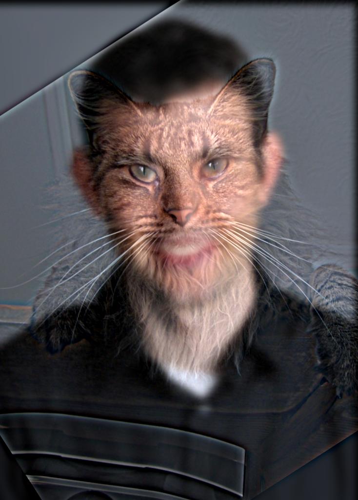
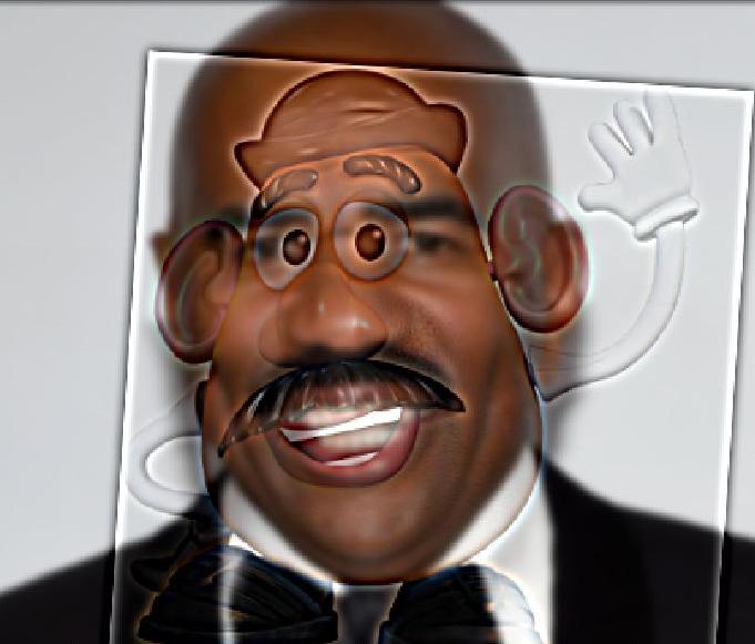
Nutmeg and Derek	Steve Harvey and Mr. Potatohead
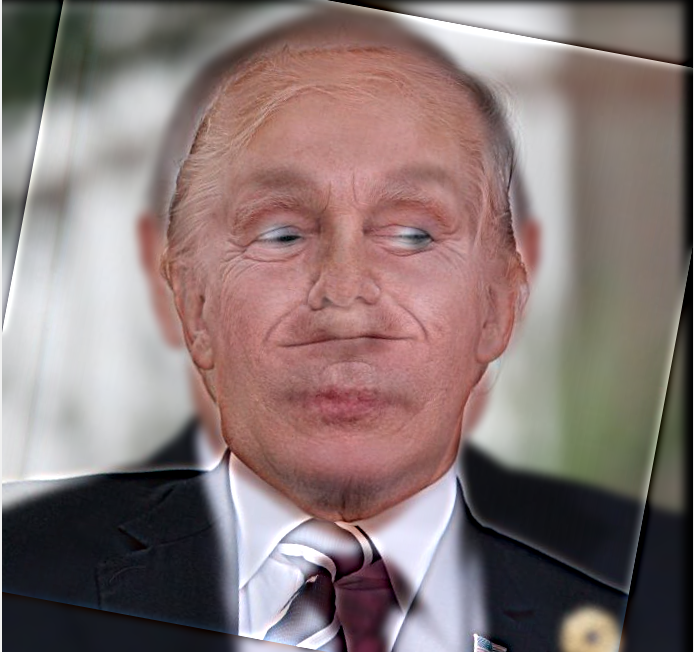
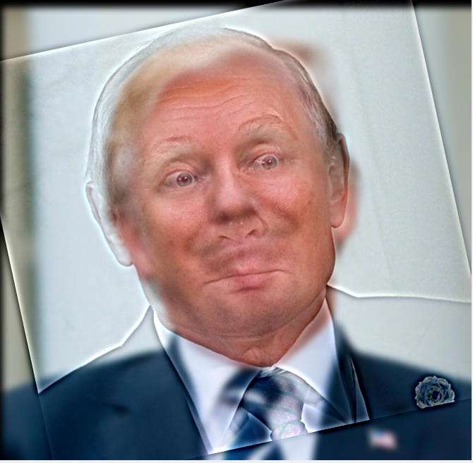
Putin Trump Fail 1	Putin Trump Fail 2

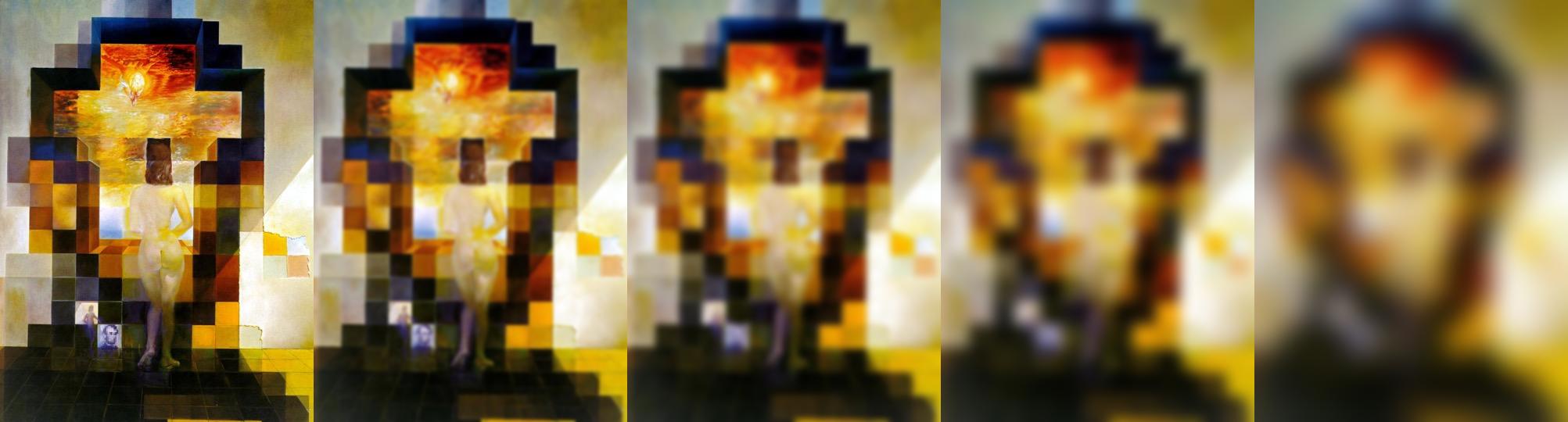
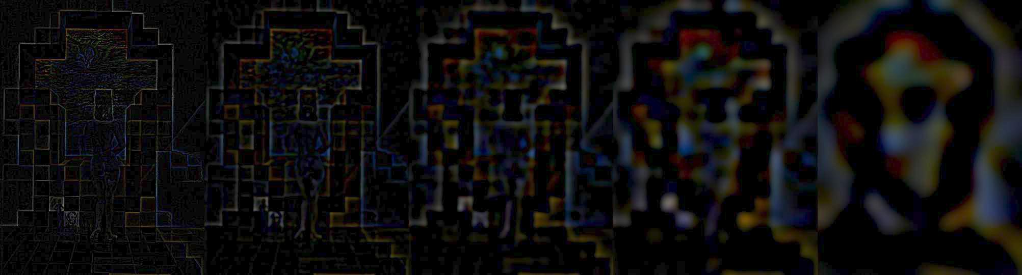
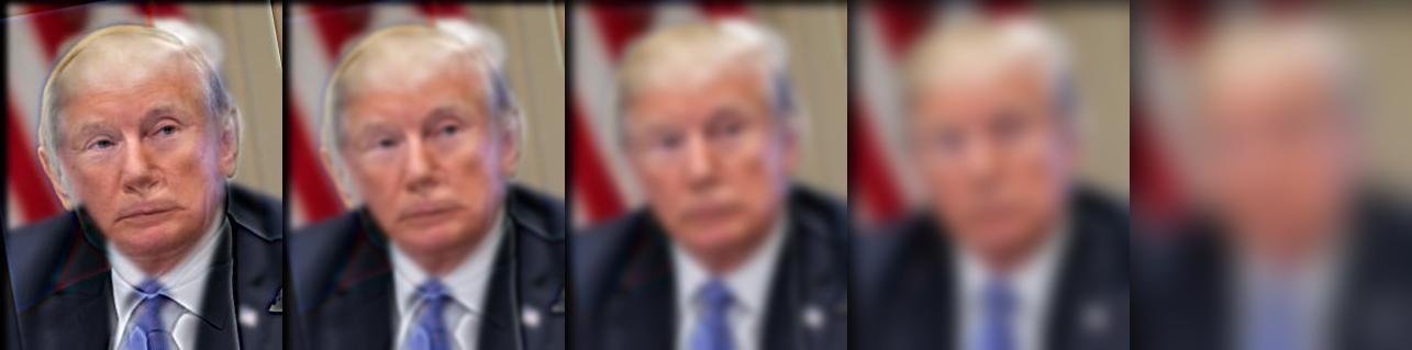
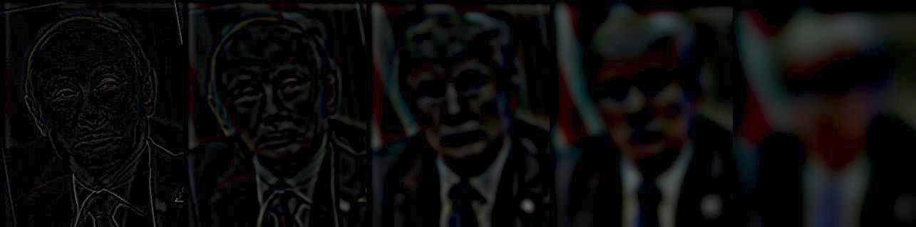
Part 1-3: Gaussian and Laplacian Stacks

The Gaussian stack is created by repeatedly applying a Gaussian filter to an image. The Laplacian stack is created by subtracting the neighboring Gaussian stack images.

Lincoln and Gala

Trump and Putin Hybrid

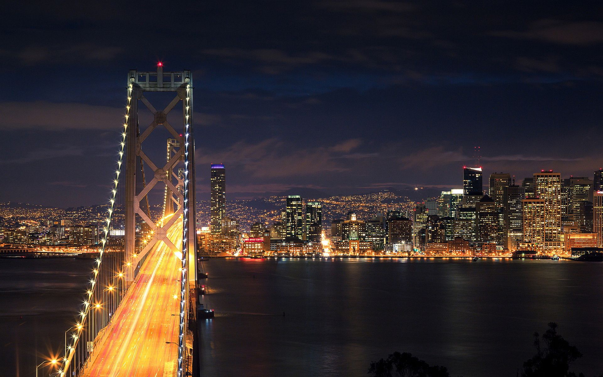
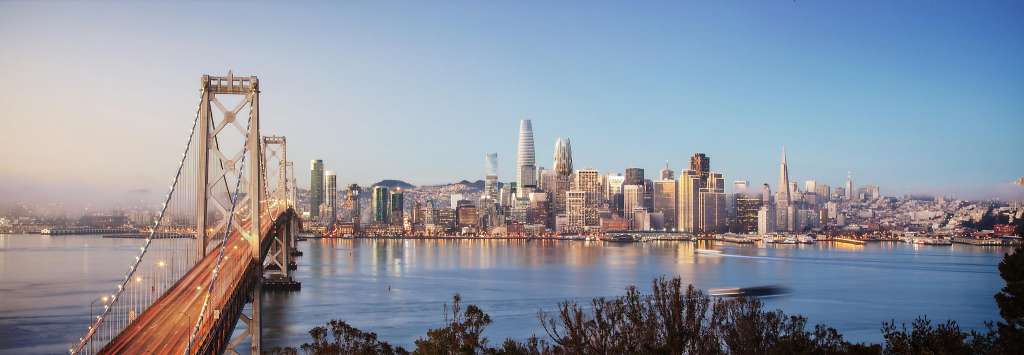
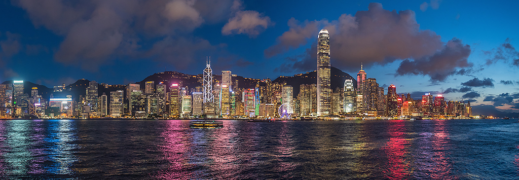
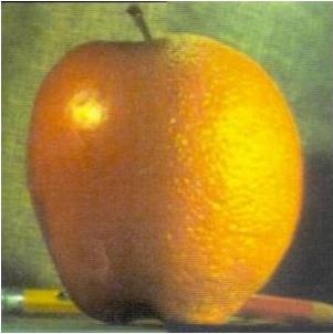
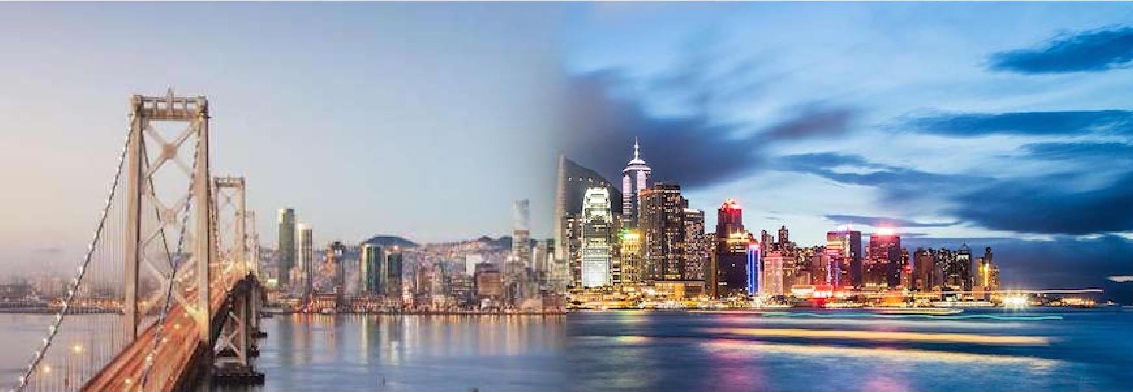
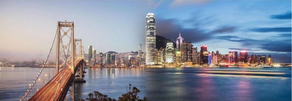
Part 1-4: Multiresolution Blending

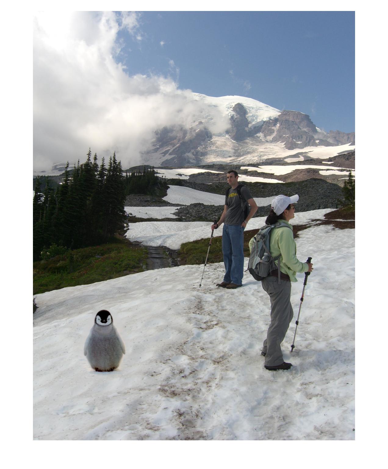
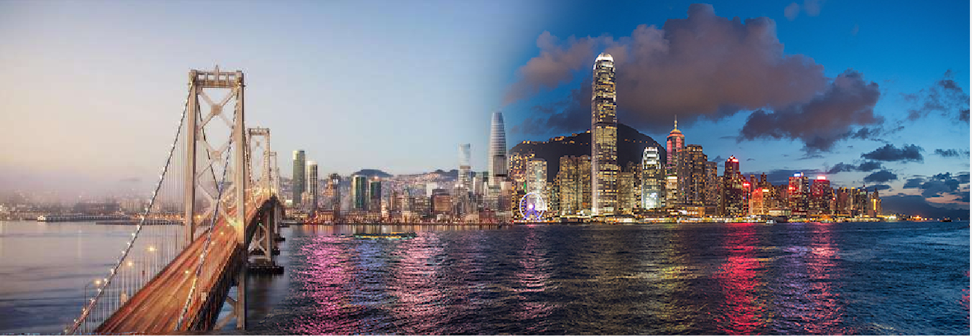
Multiresolution blending is achieved by obtaining layers of a Laplacian stack of 2 images and adding the layers back together with a mask as a separator to create a blended image.

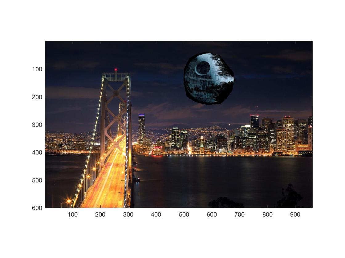
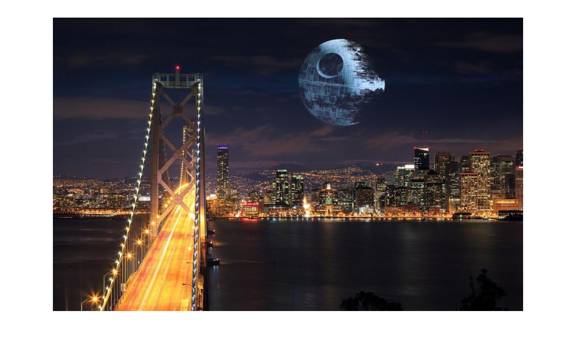
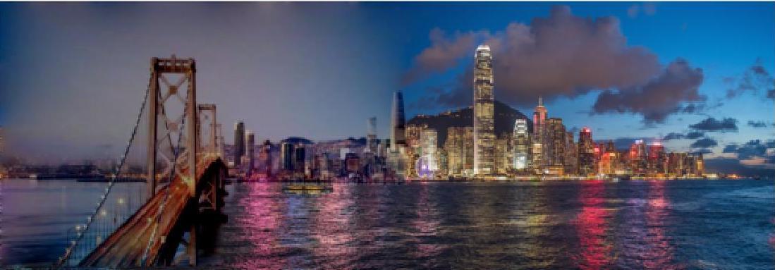
SF and Hong Kong

Blending using this mask

Blended Image

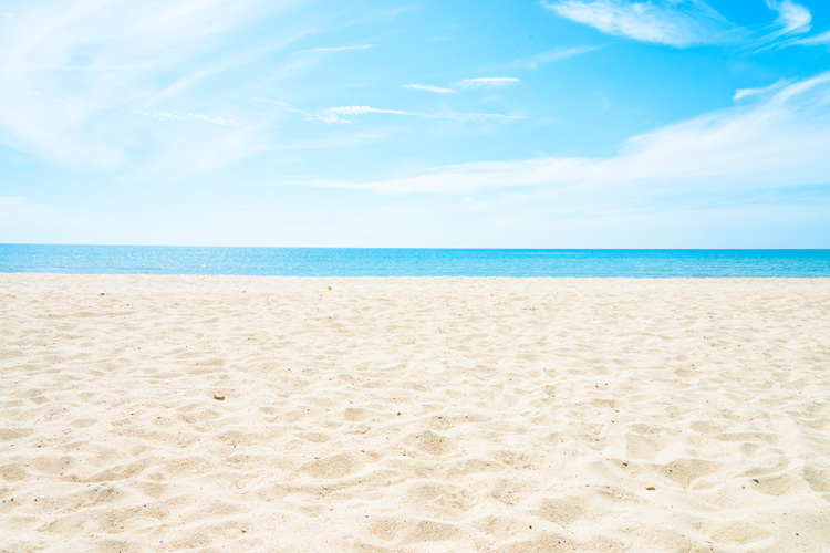
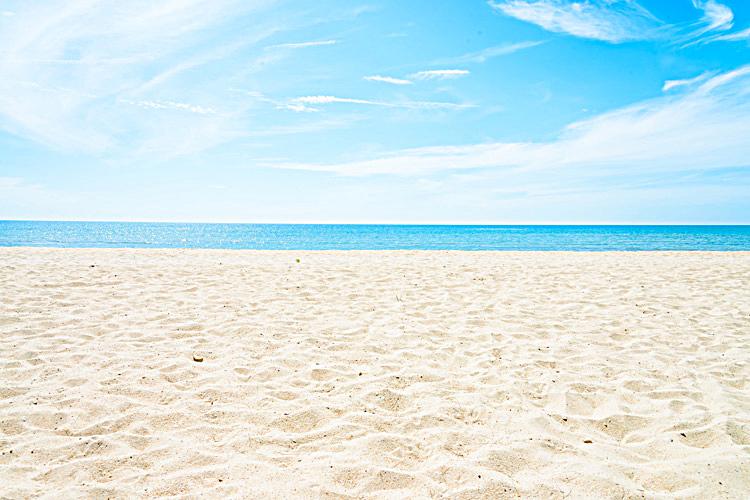
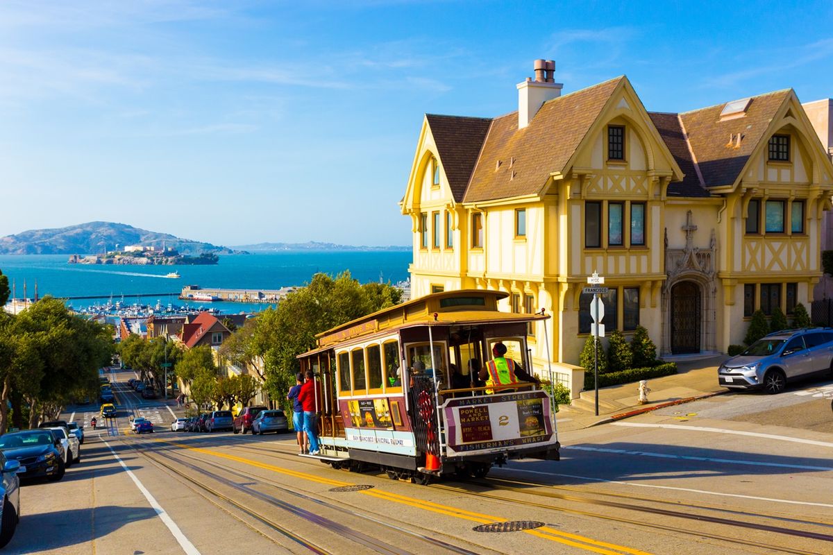
Other Blends and Attempts

Bells and Whistles

Parts 1.2, 1.3, and 1.4 all utilize color

Part 2: Gradient Domain Fusion

Overview

In this section of the project we utilize gradeitn domain fusion to blend images together. This technique is typically "better" because humans percieve the difference in gradients more than overall quality/intensity. By finding the best gradients of the source and target images to incorporate together, we can make sure the blend is smooth.
We solve for the values of overlapping pixels (source image projected on a target image) using the following formula:

's' is the source image, 't' is the target image, 'v' is the pixel values, 'i' is the location of the pixel, and 'j' is the neighbors of 'i'.

Part 2-1: Toy Problem

We reconstruct an image from its gradients by looking at its x and y neighbors and piecing together the pixel values.

Original Toy

Reconstructed Toy

Part 2-2: Poisson Blending

We blend images using the Poisson blending technique explained above.

San Fransisco	Death Star
Unblended SF + Deathstar	Blended SF + Deathstar

Other Poisson Blends

Trump + Voldemort

Penguin 1

Penguin 2

Failure

I believe this blend failed because the lighting between the two images was too drastic. Additionally, when Matlab adjusted the Mario image, it believed there was a black background despite the image having no real background. The blending thought Mario was too dark and scaled up the pixel values, which made the final image a failure.

Laplacian Pyramid Blending vs Poisson Blending

The Laplacian Pyramid Blending is clearly better than the Poisson Blending. This is because the lighting between the two images is too drastic - the picture of SF is in the daytime and the picture of Hong Kong is nightime. The Poisson blend tries to blend more of the whole image, whereas the Laplacian Pyramid really only blends the edges of the mask, which preserves lighting and quality.