Fun with Frequencies and Gradients
CS194-26 Image Manipulation and Computational Photography
Jingxi Huang cs194-26-aap
Overview
The goal of the project is to create sharpened images by using the unsharp masking technique, to construct hybrid
images by combining the low and high frequencies of two different images, to blend multi-resolution images using
Gaussian and Laplacian stacks and finally to seamlessly blend an object or texture from a source image into a target
image using poisson blending.
Part 1: Frequency Domain
Part 1.1: Unsharp Masking
To create the sharpening effect, I used the unsharp masking technique. For an image f and a Gaussian filter g, we
can create a blurred image f * g and get the details of the image f - f * g by subtracting the blurred image from
the original image. Then, we accentuating the high frequencies of the image by adding a times the detail of the image
so that we get the sharpened image f + a(f - f * g)). In the following example, I choose the filter size half width
to be approximatlely 3 * sigma when creating the gaussian filter.
 original image
|
 blurred image
|
 detailed image
|
 sharpened image
|
 original image
|
 blurred image
|
 detailed image
|
 sharpened image
|
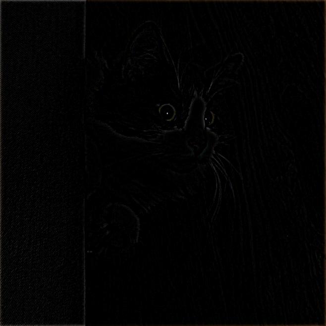
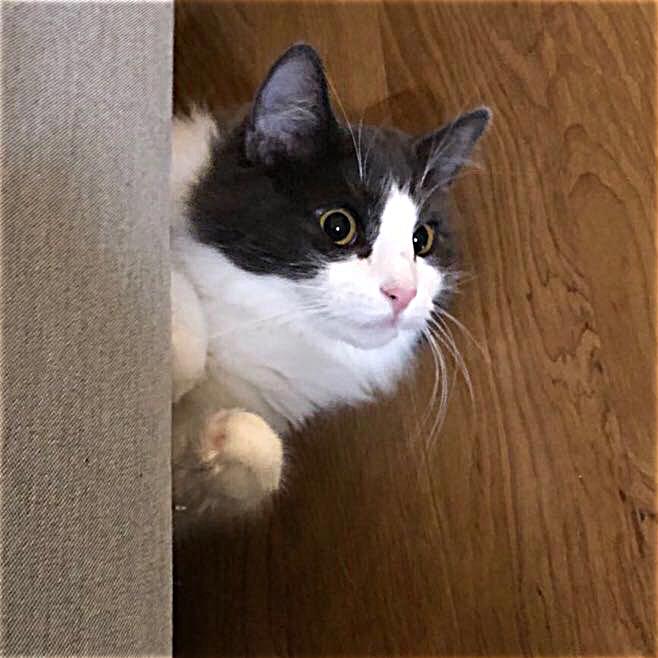
Part 1.2: Hybrid Images
Hybrid images are static images that change in interpretation as a function of the
viewing distance. The basic idea is that high frequency tends to dominate perception
when it is available, but, at a distance, only the low frequency (smooth) part of the
signal can be seen. By blending the high frequency portion of one image with the low-frequency
portion of another, you get a hybrid image that leads to different interpretations
at different distances.
To create hybrid images, we combined the low pass portion of one image(a blurred image f * g
where g is the gaussian filter) with the high pass portion of another image(a Laplacian f - f * g).
By adding them up, we get our hybrid image.
1.2.1 Derek + Nutmeg
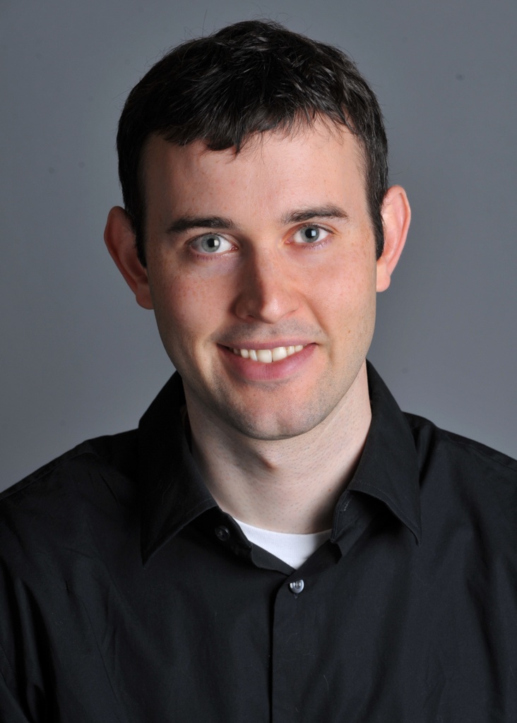 derek.jpg
|
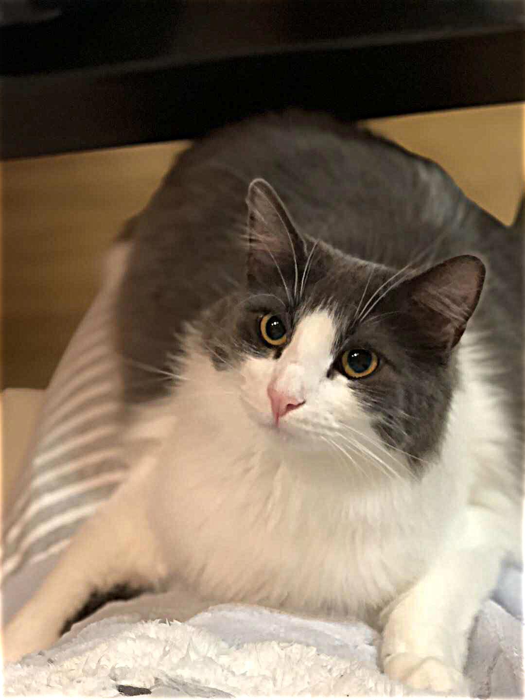
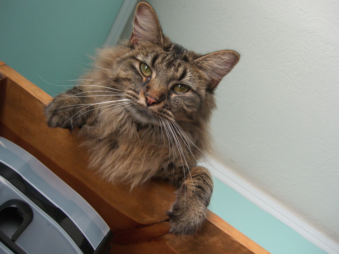 nutmeg.jpg
|
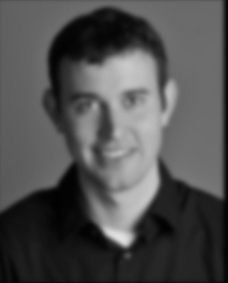 low frequency derek
|
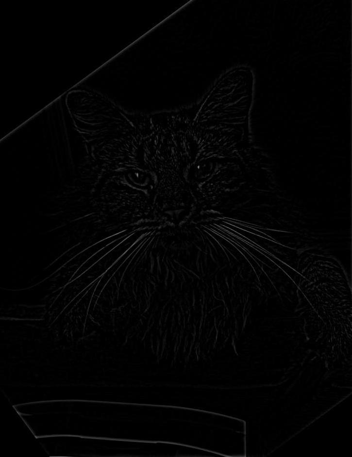 high frequency nutmeg
|
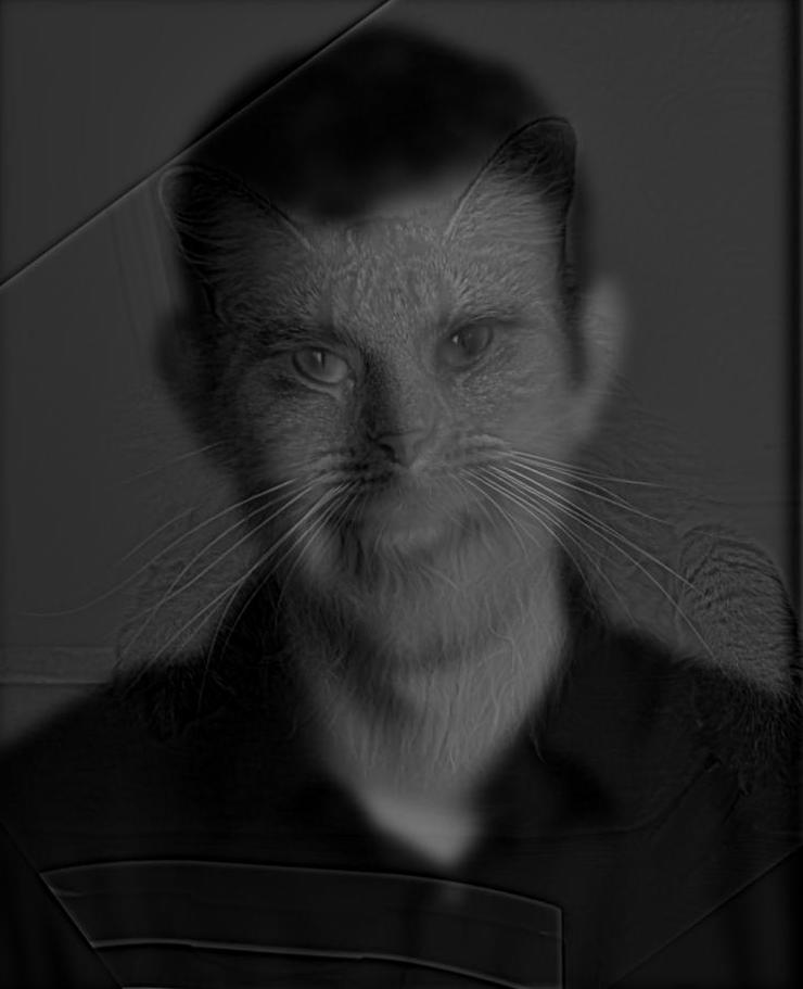 hybrid derek and nutmeg in gray
|
Bells & Whistles
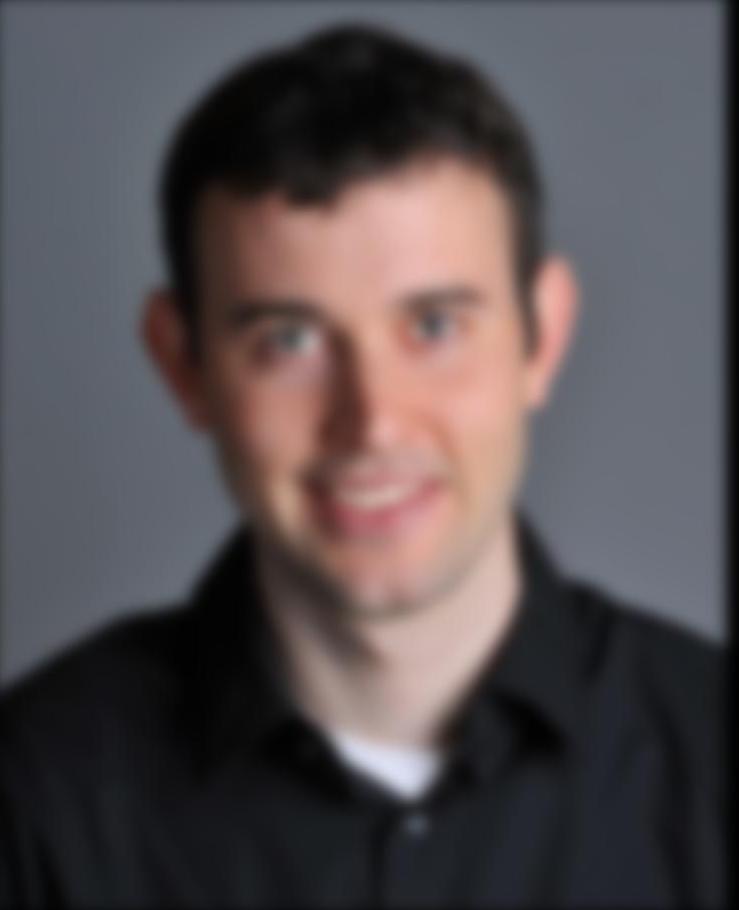 low frequency derek
|
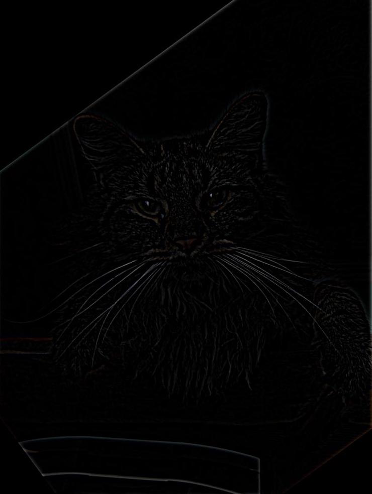 high frequency nutmeg
|
 hybrid derek and nutmeg in color
|
1.2.2 More Results
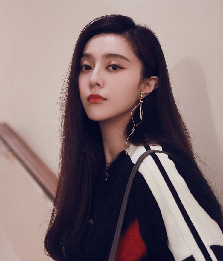 Bingbing Fan
|
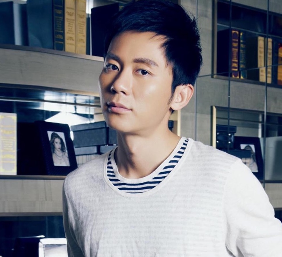 Chen Li
|
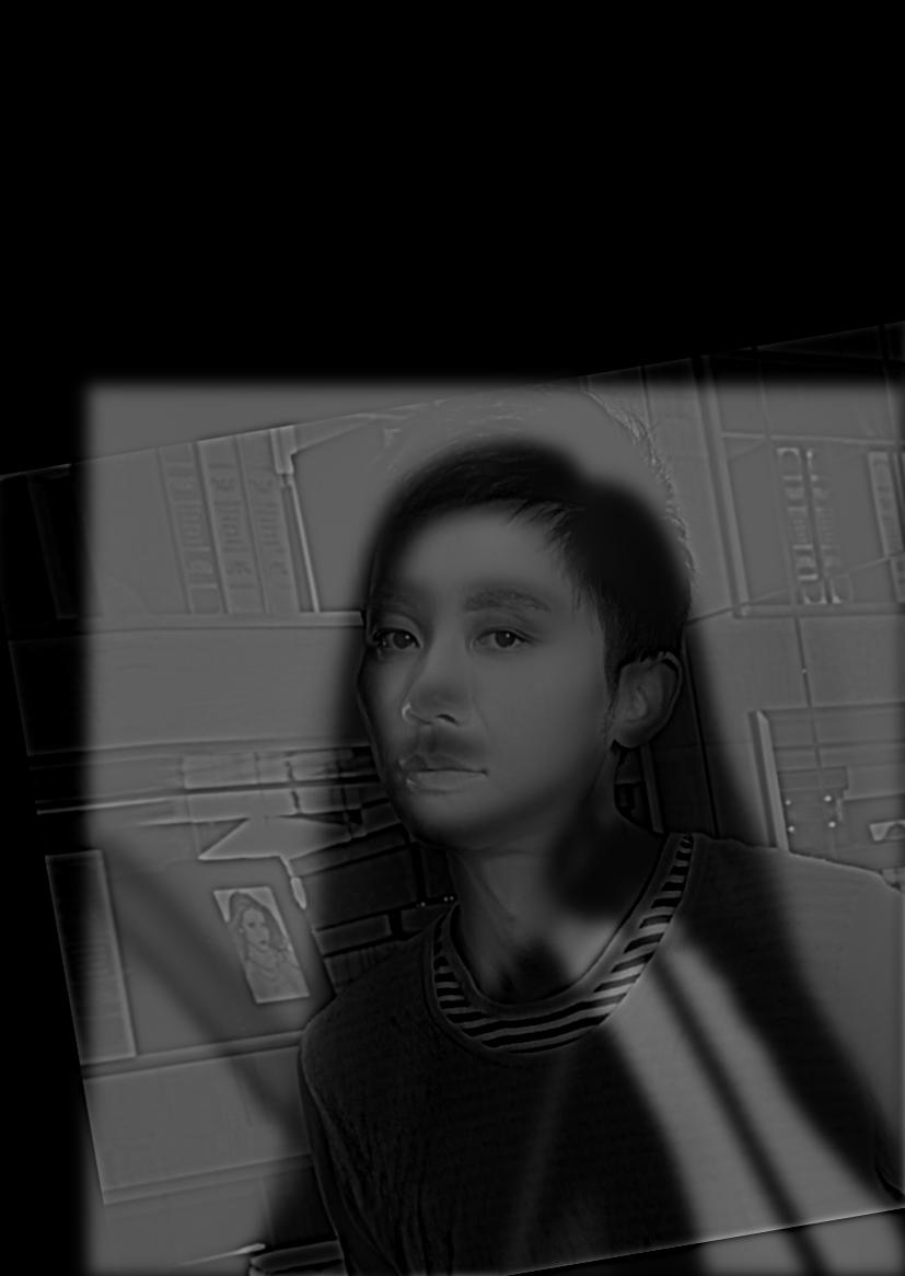 hybrid in gray
|
 hybrid in color
|
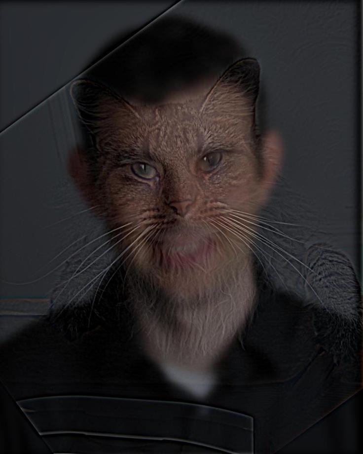
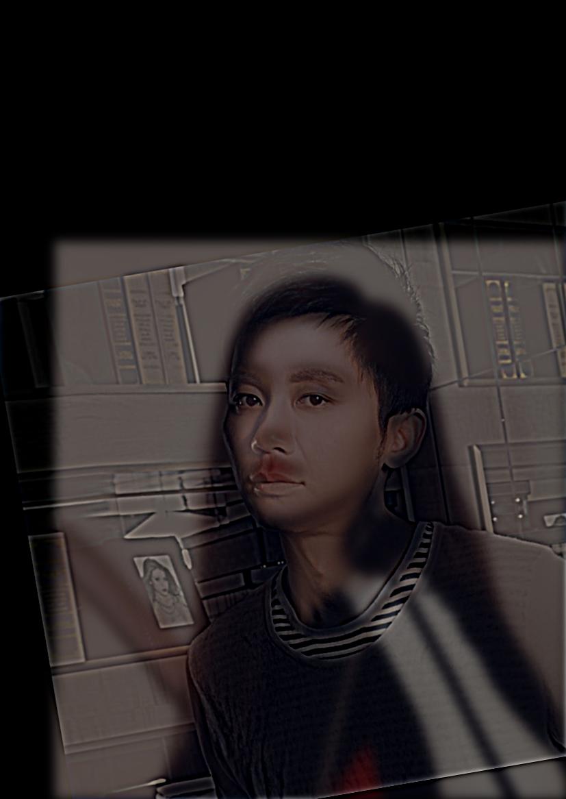
 Jason Statham
|
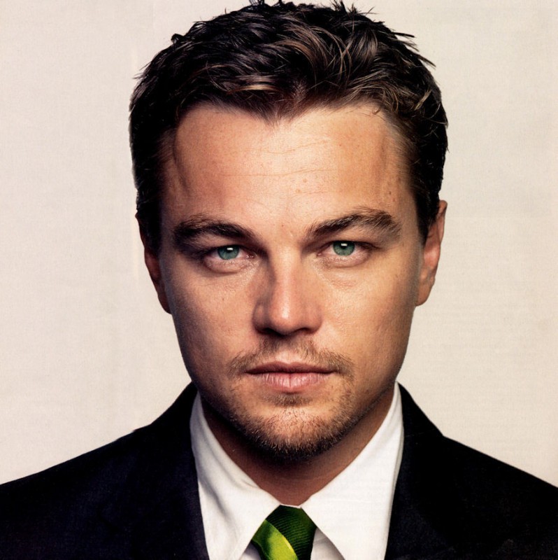 Leonardo DiCaprio
|
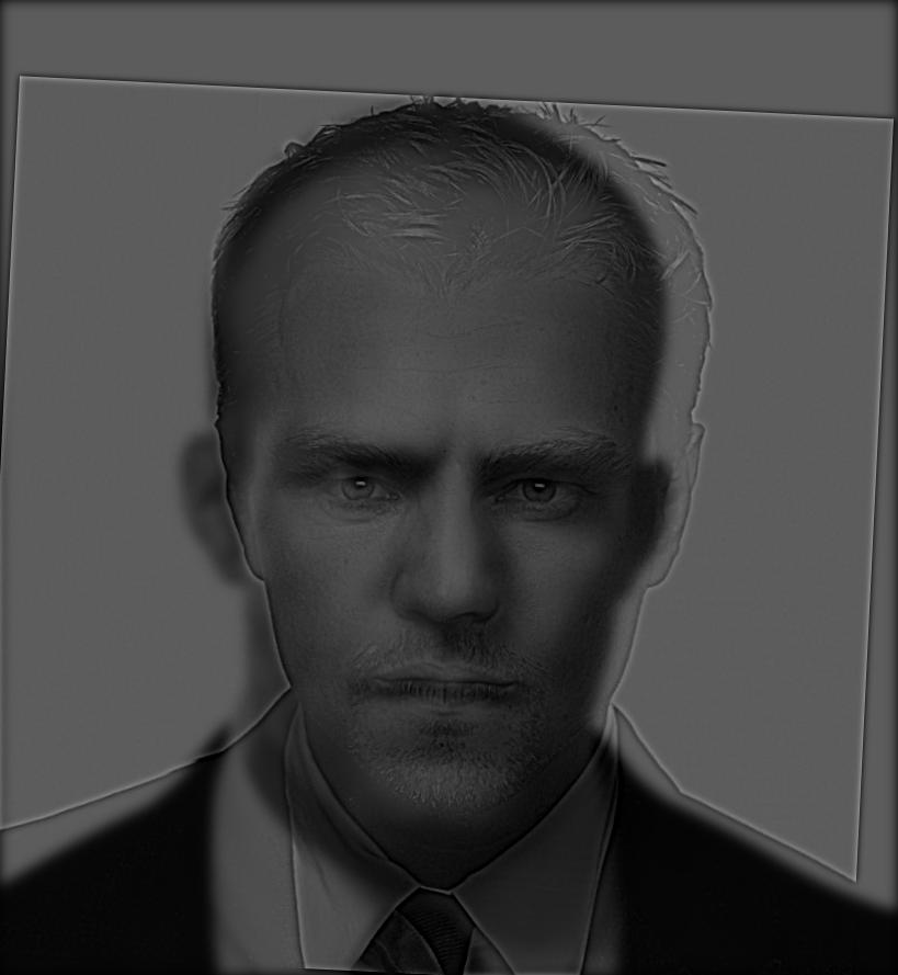 hybrid in gray
|
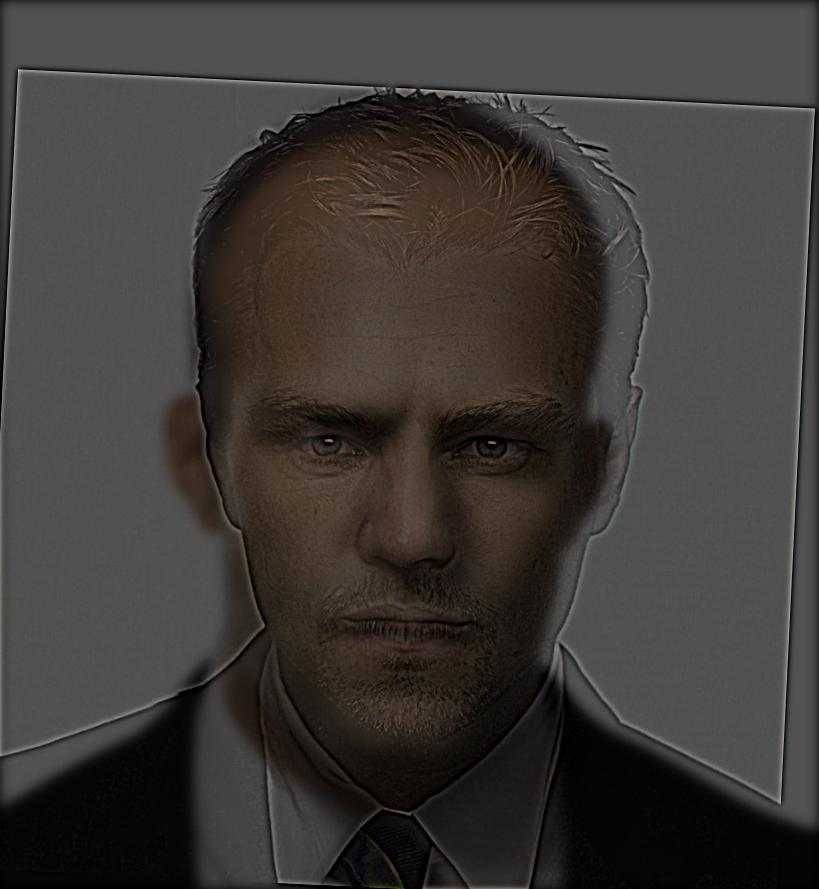 hybrid in color
|
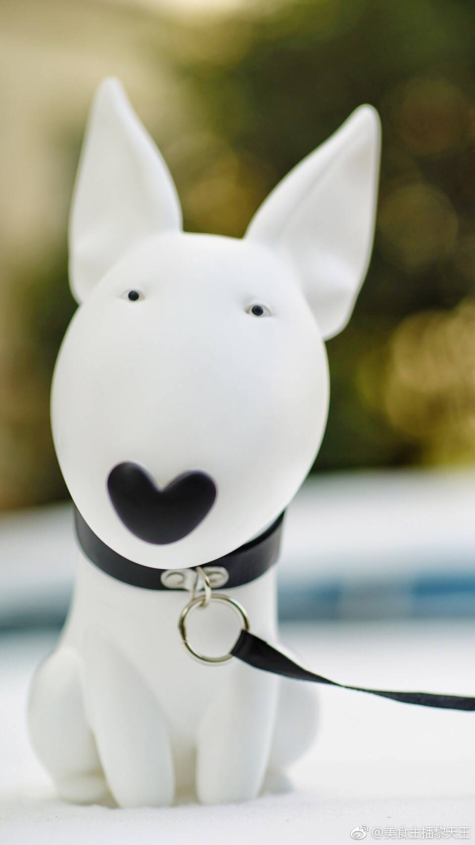 dog
dog
|
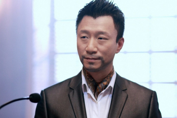 Honglei Sun
|
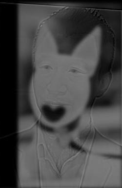 hybrid in gray
|
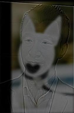 hybrid in color
|
1.2.3 Failure Result
The following hybrid isn't that succesful since the background of Corgi is too bright so that we
couldn't see the Husky very clearly when we are close to the image.
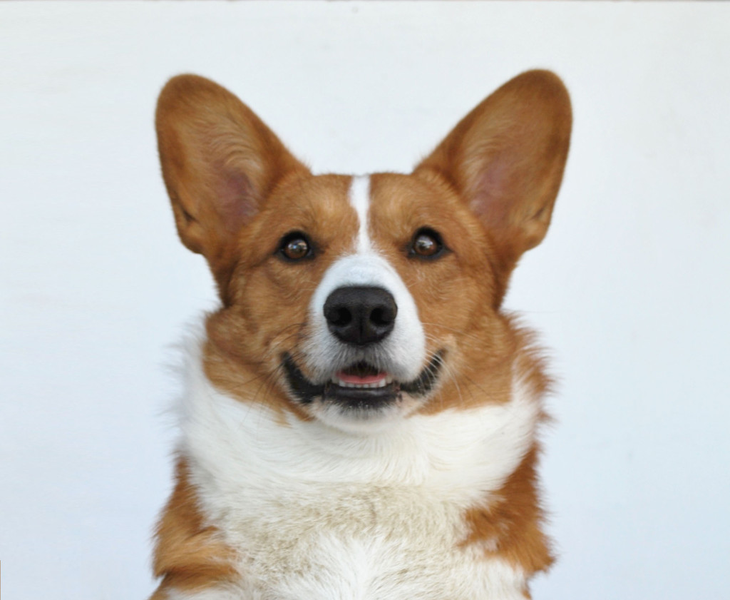 Corgi
Corgi
|
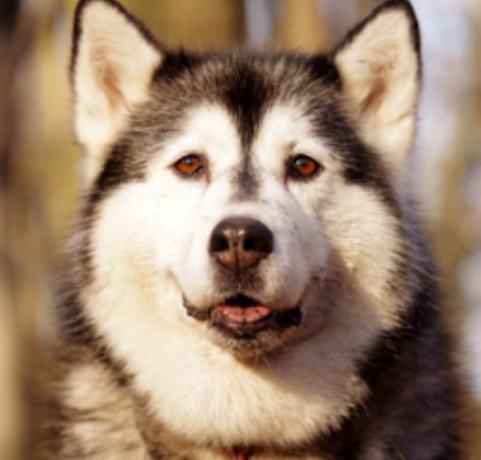 Husky
Husky
|
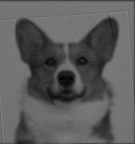 hybrid in gray
|
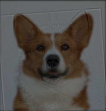 hybrid in color
|
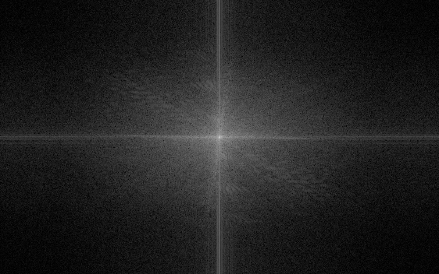
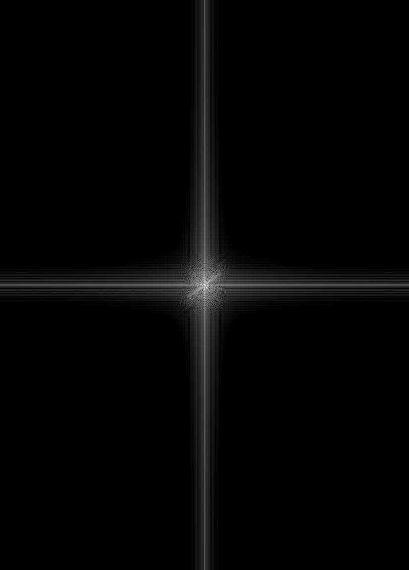
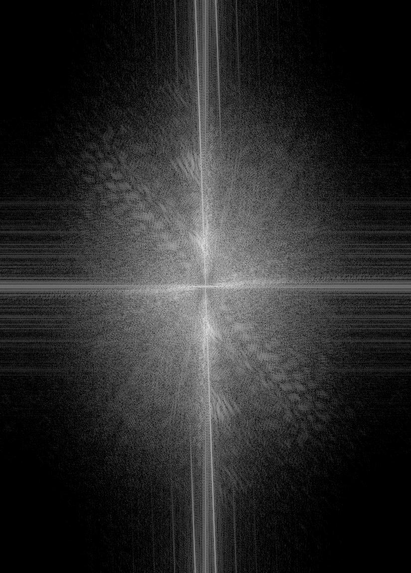
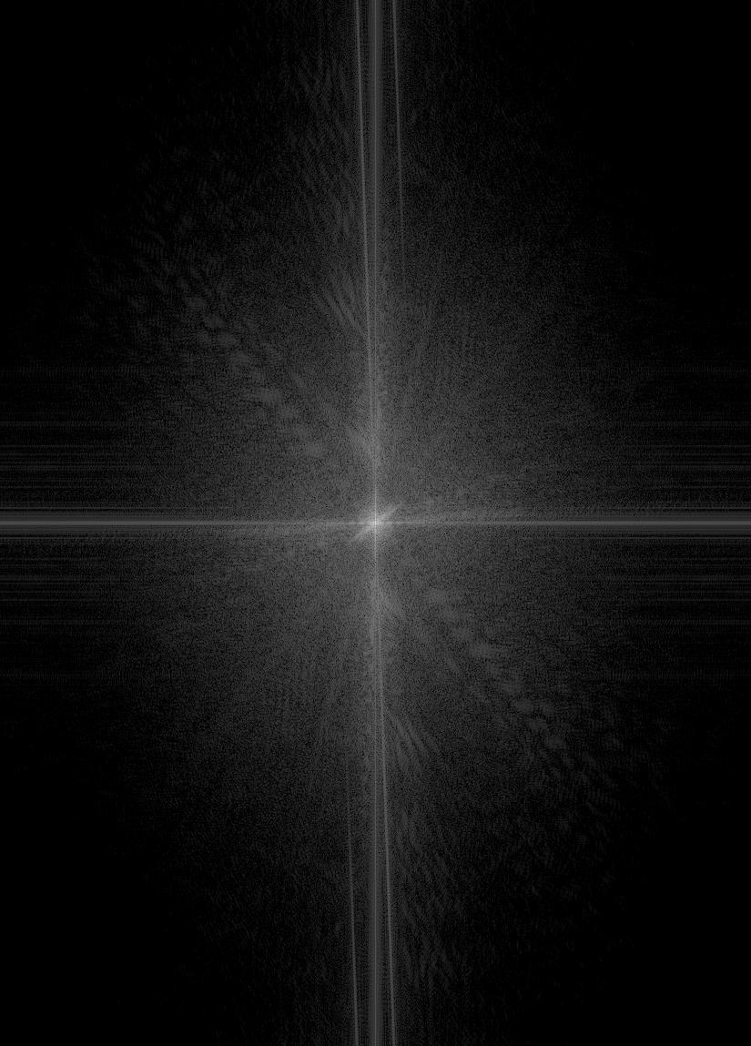
1.2.4 Frequency Analysis
Below are the log magnitude of the Fourier transform of the two input images, the filtered images, and the hybrid image.
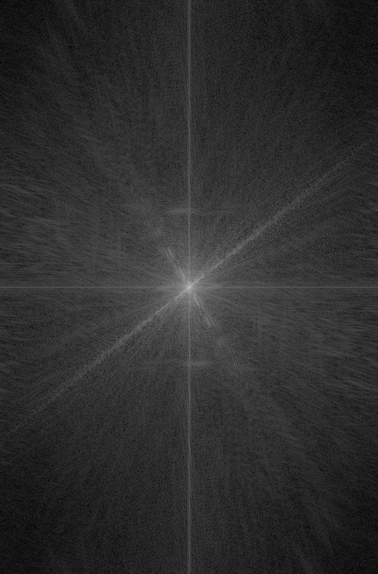 Bingbing Fan
|
 Chen Li
|
 low pass Bingbing Fan
|
 high pass Chen Li
|
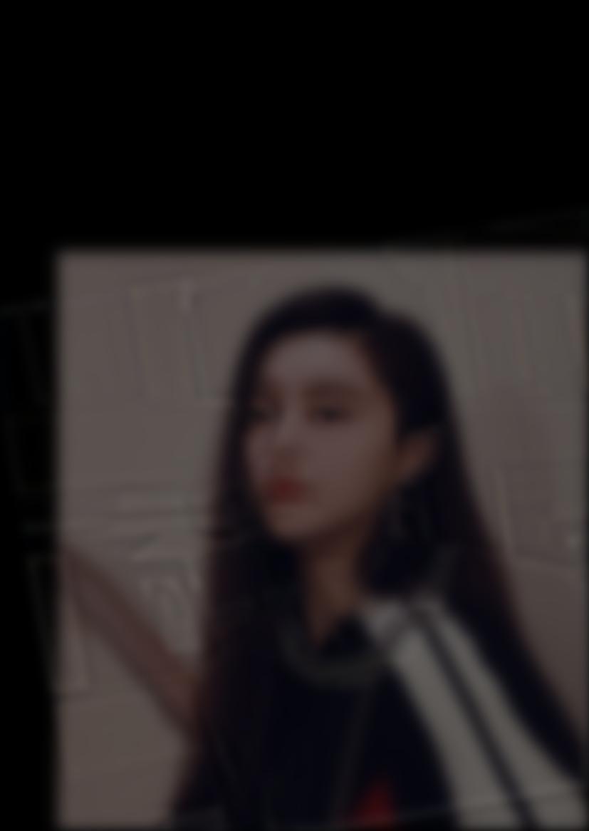
 hybrid result
|
Part 1.3: Gaussian and Laplacian Stacks
By repeatedly applying a Gaussian filter with increasing size on the image, we get the Gaussian stack.
After that, a Laplacian stack stores the difference between each two Gaussian stack and the last layer of
Laplacian stack is the same as the last layer of Gaussian stack.
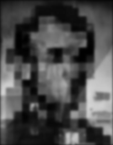
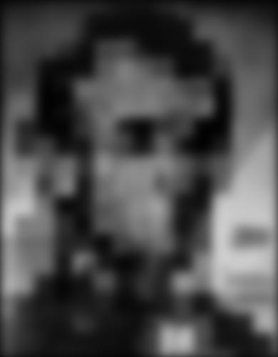
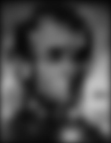
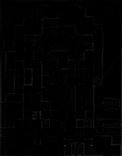
1.3.1 Lincoln
Lincoln Gaussian Stack
Lincoln Laplacian Stack
1.3.2 Hyrbrid Image of Bingbing Fan, Chen Li
Hybrid Gaussian Stack
Lincoln Laplacian Stack
Part 1.4: Multiresolution Blending
In order to blend two images seamlessly using a multi resolution blending, we compute the Gaussian
stack GR for a given mask and Laplacian pyramids LA and LB for both images. Then we form the combined
pyramid LS by using the pyramids we constructed and for each level, we have LS(i, j) = GR(i, j)LA(i, j) + (1 - GR(i, j))LB(i, j).
Finally, we can reconstruct the image by adding all the layers together.
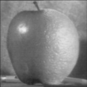
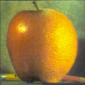
1.4.1 Orange + Apple
 Apple
Apple
|
 Orange
|
 blending image in gray
|
 Bells & Whistles: color blending
|
1.4.2 Candy + Candy
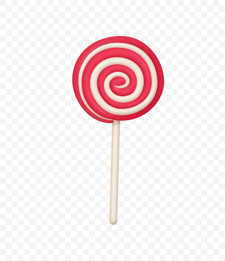 Candy
Candy
|
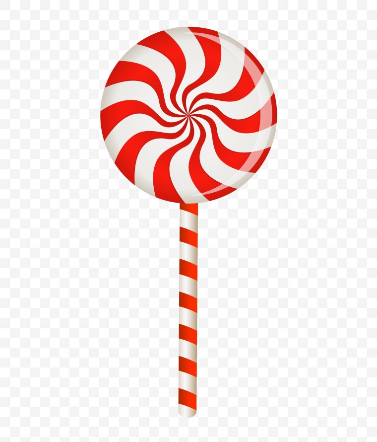 Candy
Candy
|
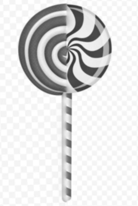 blending image in gray
|
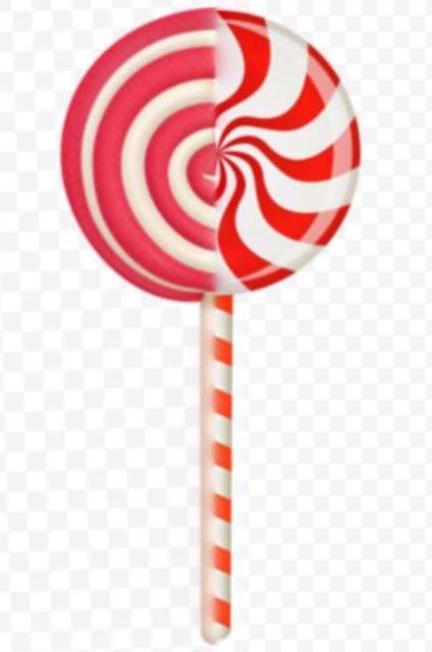 Bells & Whistles: color blending
|
1.4.3 Irregular Mask: Sky + rainbow
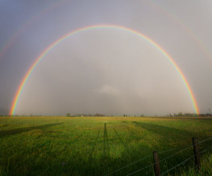 Source Image
|
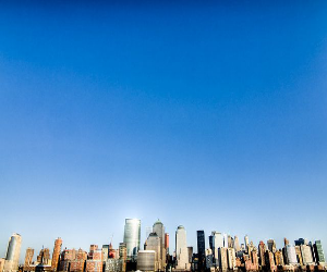 Target Image
|
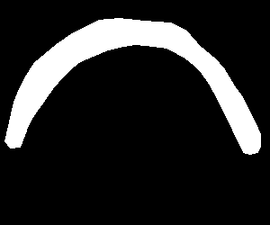 Mask
Mask
|
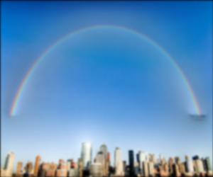 Laplacian Pyramid Blending
|
Part 2: Gradient Domain Fushion
The primary goal of the second part of the project is to seamlessly blend an object or texture from a
source image into a target image. Our goal was to implement gradient-domain blending, in which we blended
an object from a source image s to a target image t. Instead of directly copying the pixels of source
image, which will lead to unnatural blending due to the different color tone between source and target
image, we are going to implement poisson blending.
To implement the blending, we are going to solve the optimization with two constraint. First, we want the
gradient of the target portion to be as similar as that of the source. Second, we want the similar gradient
around the boundary so that we won’t see sharp edges.
Part 2.1: Toy Problem
By solving the x-gradients of v should closely match the x-gradients of s, the y-gradients of v should
closely match the y-gradients of s for each pixel as well as keeping the top left corners of the two images
should be the same color, we reconstruct the orignal image as shown below.
 Original Image
|
 Reconstructed Image
|
Part 2.2: Poisson Blending
Part 2.2.1 Poisson blending results
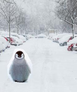
Penguin + Snow
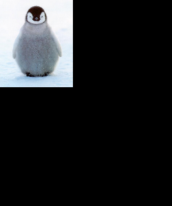 Source Image
|
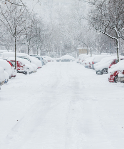 Target Image
|
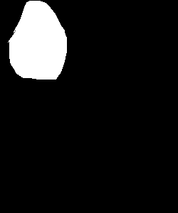 Source Mask
|
 Target Mask
|
 Direct Copy
|
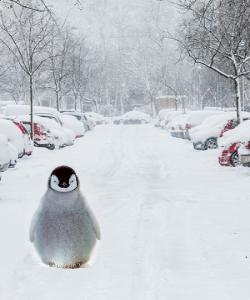 Poisson Blending
|
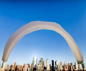
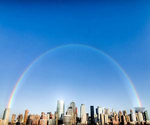
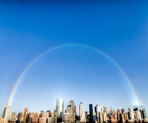
Rainbow + Sky
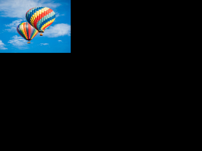 Source Image
|
 Target Image
|
 Source Mask
|
 Target Mask
|
 Direct Copy
|
 Poisson Blending
|
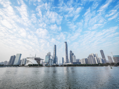
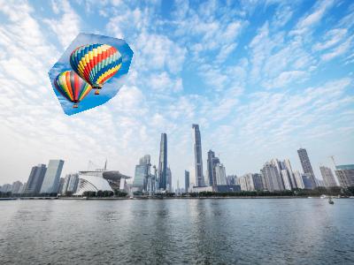
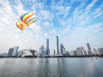
UFO + City
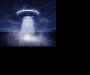 Source Image
|
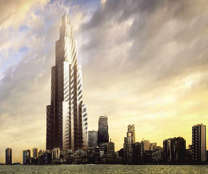 Target Image
|
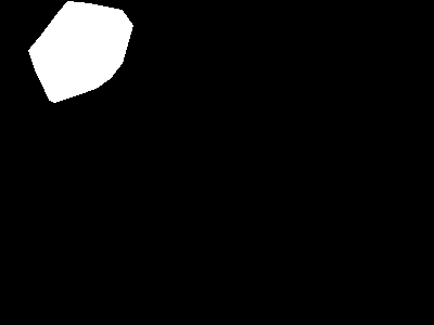
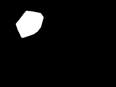
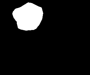 Source Mask
|
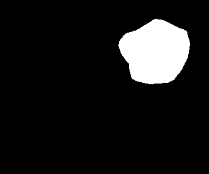 Target Mask
|
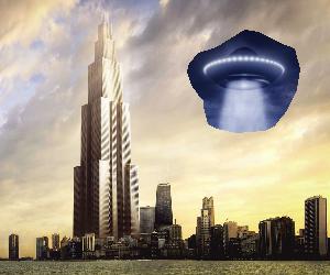 Direct Copy
|
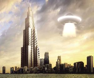 Poisson Blending
|
Part 2.2.2 Poisson blending failures
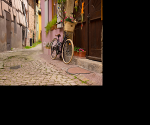
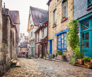
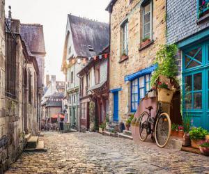
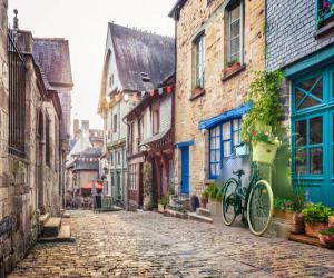
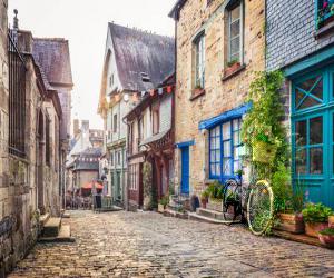
Street + Bicycle
Poisson blending fails in this case becasue the background of the source and target images are very different
in the blue door. Also since the target has a background pattern that is different from the pattern of the source,
poisson blending can only blend with the color but not create similar pattern in the target image.
 Source Image
|
 Target Image
|
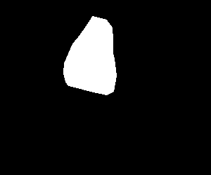 Source Mask
|
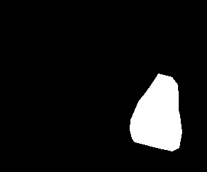 Target Mask
|
 Direct Copy
|
 Poisson Blending
|
Bells & Whistles: Mixed Gradient
This is an example of using mixed gradient.The result is better than the poisson Blending
since mixed gradient takes into account of both source image gradient si-sj and target image gradient
ti-tj at the boundary of the portion that we want to blend. So that we will be able to keep some of
the background pattern when doing the blending.
|
Source Image
|
Target Image
|
Direct Copy
|
Poisson Blending
|
 Mixed Gadient
|
Part 2.2.2 Blending techniques comparison
In the following example, we can comparing the result of direct copy, laplacian pyramid
blending, poisson blending and mixed gradient techniques. We can see that direct copy has the worst result
since we will get very unnatural boundaries in the resulting image. In this case laplacian
pyramid is also not working very well since the color of the source and target images are
very different. Poisson blending works better because one of the constraint of poisson blending
is to keep the gradient near the boundary to be small. Since the sky is pure in this case,
poisson blending works well by making the boundary the same as that of the target image. For mixed
gradient, the result is similar to poisson blending since there are not much pattern in the background
of the target image so both techniques are working very well.
|
Source Image
|
Target Image
|
 Direct Copy
|
LP Blending
|
 Poisson Blending
|
 Mixed Gradient
|
The Program
To run the program, put input images under corresponding directories, run
python3 main.py sharpen img.jpg
python3 main.py hybrid img1.jpg img2.jpg
python3 main.py stack img.jpg
python3 main.py blend img.jpg
python3 poisson_blending.py img1.jpg img2.jpg