CS 194-26: Image Manipulation & Computational Photography
Project 3: Frequencies and Gradients
Blurring, blending and more
Barbara Yang, cs194-26-aar
Overview
Project specs
FILL IN THIS PART
Part 1: Frequency Domain
Part 1.1: Warmup
As a warmup, I implemented a low-pass filter using a Gaussian kernel and used it to sharpen an image. This is
also called an unsharp masking technique.
Procedure
- Create a Gaussian kernel (source)
using a chosen
sigma
- Convolve the kernel with your image array
- Trim artifact borders from convolved result
- Subtract original image and trimmed, convolved Gaussian image
- Add the difference and the original image
By finding the difference between the blurred and original images, I isolated the areas of highest frequency
(i.e.
details). Then, by adding these pixels back into the original image, I can emphasize the details, creating a
sharpened effect.
Results

Slightly blurry photo of my dog, Ginger
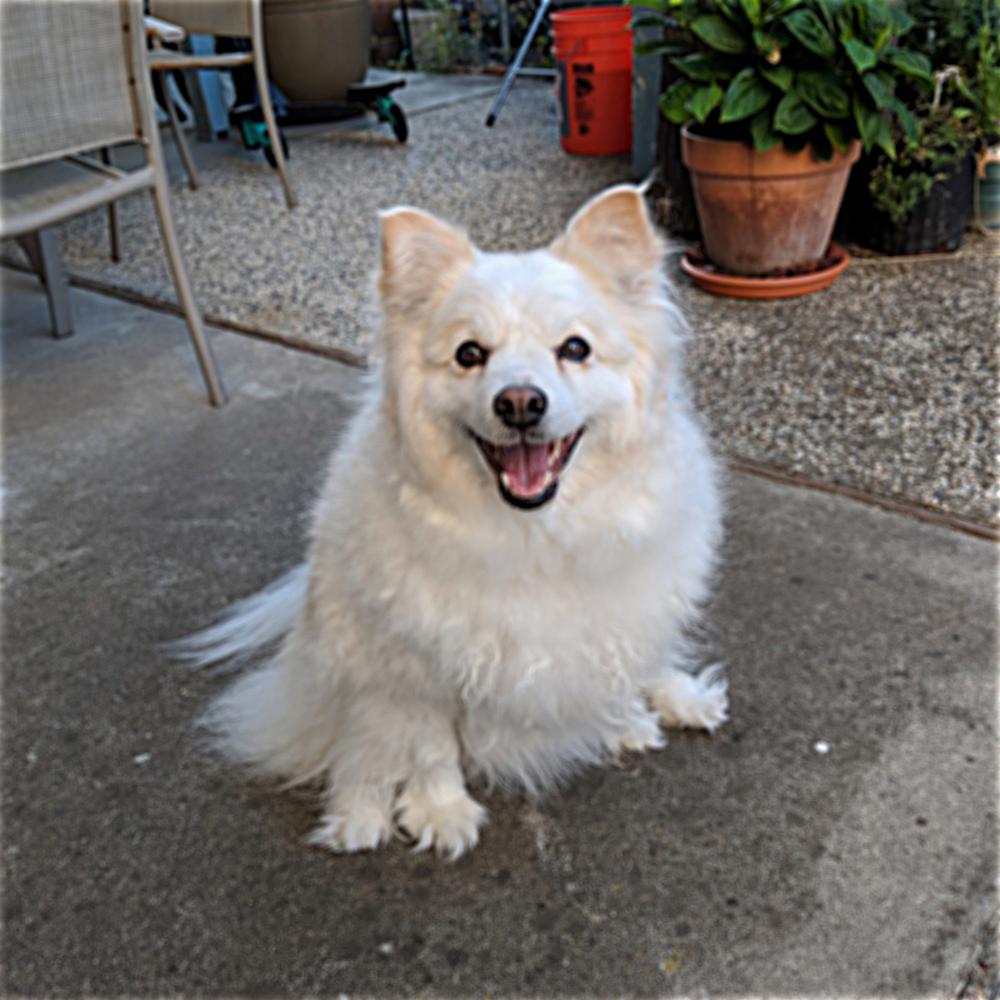
Sharpened image, sigma = 20

Sharpened image, sigma = 50
Part 1.2: Hybrid Images
In an more involved exercise, I created hybrid images by combining two images treated with a high or low pass
filter. The high pass filter isolates sharp details while the low pass filter gives a lburry photo represented by
patches of light or dark areas. The optical illusion is that the viewer sees two different images from near and
far distances.
Procedure
- Obtain two images with similar poses, silhouettes and scaling.
- Convolute a Gaussian kernel with the first image to isolate its low frequencies (blurry image).
- Convolute a Gaussian kernel with the second image. Then, subtract the image with the convoluted result. This
gives the high frequences of the second image (details and edges).
- Add together the low and high frequency images
Results

Tiger cub
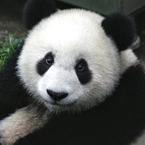
Panda

Piger / tanda

Very spherical apple

Mini watermelon
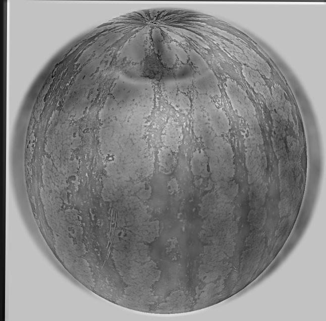
Applemelon
Failure case

Adult golden retriever

Puppy golden retriever
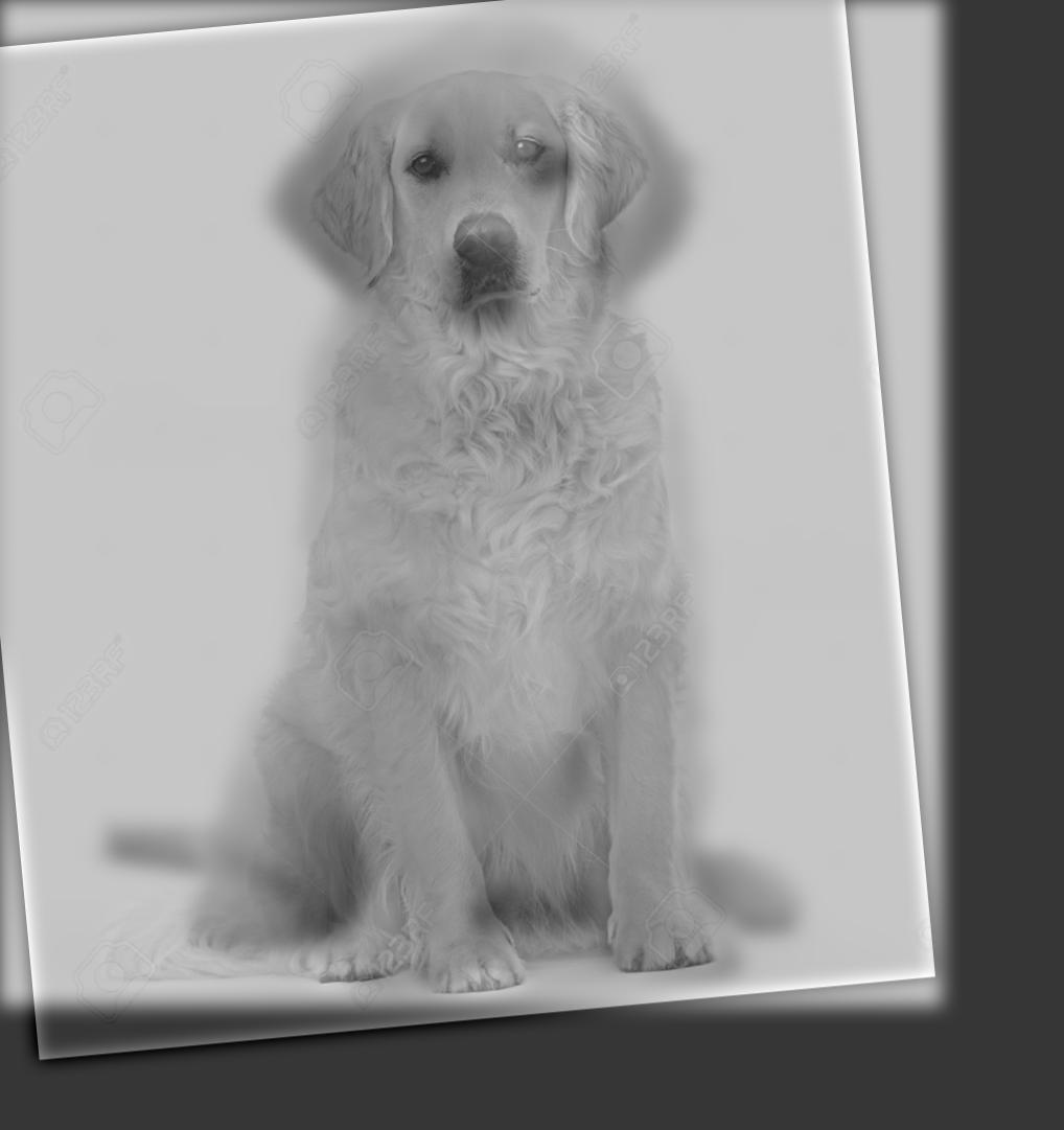
Bad combination due to mismatch of body proportions (note head-to-body ratio)
Fourier analysis
For the "Watermelon/Apple" case, I produced a Fourier analysis using the provided code, np.log(np.abs(np.fft.fftshift(np.fft.fft2(gray_image)))),
where gray_image is a grayscale (luminance channel) version of each image.
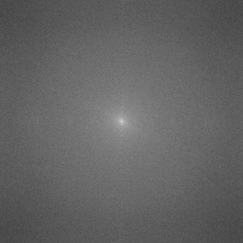
Apple

Watermelon

Low freq
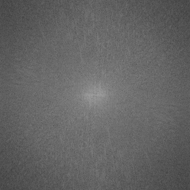
High freq

Result
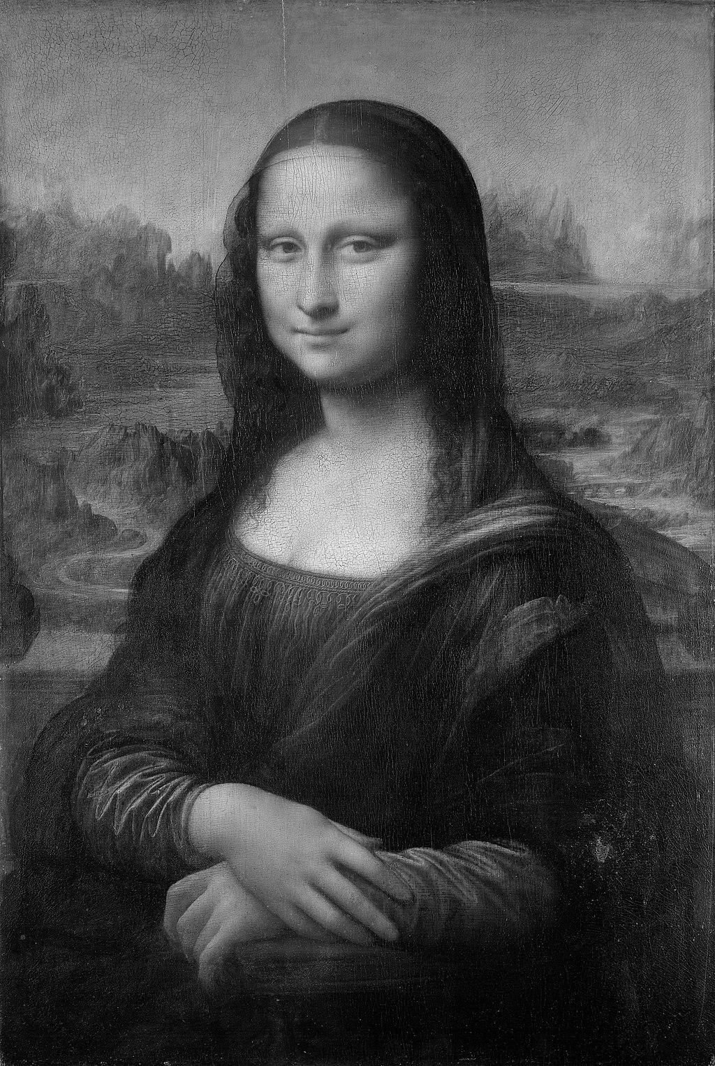
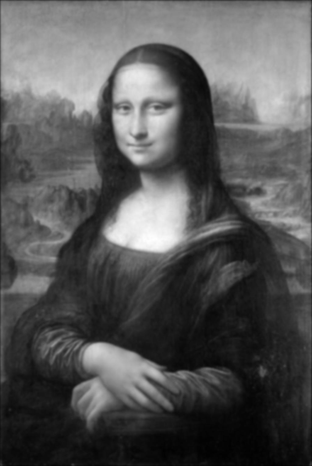
Part 1.3: Gaussian and Laplacian Stacks
Next, I created image stacks to analyze the structure of images at different "resolution" levels. Every image in
a Gaussian stack is the same dimension (so we do not downscale, as in a pyramid). However, each one uses an
exponentially larger σ (I used ** 1.3) than the previous level. In a Laplacian stack, each
image is the difference between two adjacent levels of a Gaussian stack.
Mona Lisa - Gaussian stack
Mona Lisa - Laplacian stack

L0 = G0 - G1

L1 = G1 - G2

L2 = G2 - G3

L3 = G3 - G4

L4 = G4
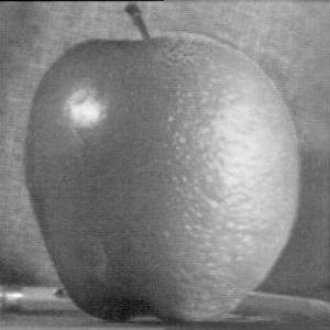
I also revisit my hybrid watermelon/apple from earlier. The Gaussian and Laplacian stacks also reveal a pattern
about the hybrid image. Specifically, the lower levels of the Laplacian stack highlight the high-pass differences.
Hybrid - Gaussian stack
Hybrid - Laplacian stack

L0 = G0 - G1
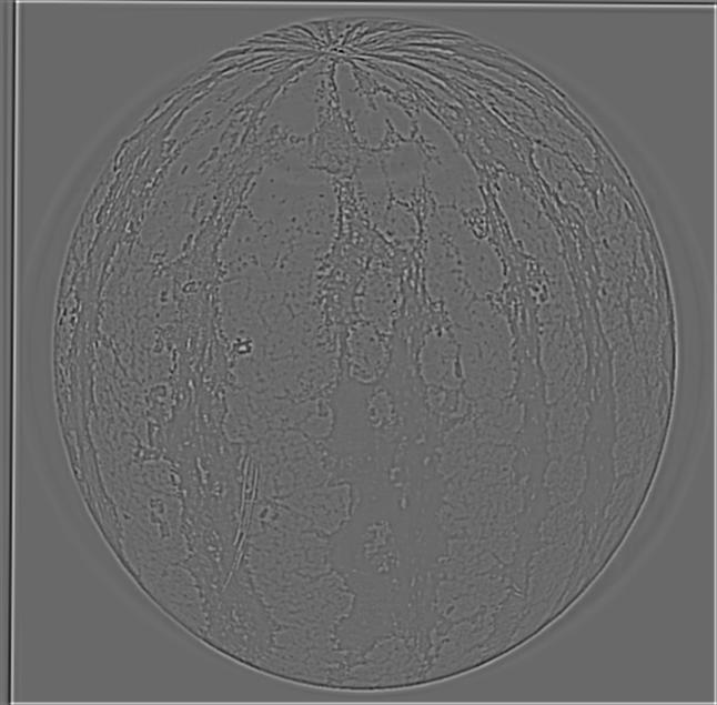
L1 = G1 - G2
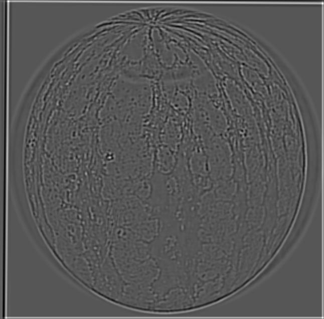
L2 = G2 - G3
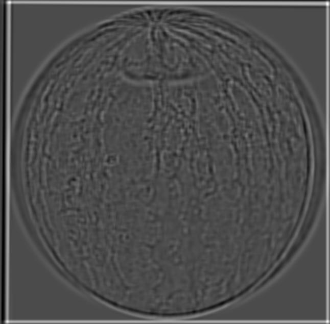
L3 = G3 - G4

L4 = G4
Part 1.4: Multiresolution Blending
In a Laplacian stack, each level captures different amounts of detail. I can use this to create a smooth blend
between two photos, where the finest detail uses a sharp mask and the most general color areas use a blended mask.
Procedure
- Obtain two images of the same dimensions.
- Create a binary mask (black and white) of the same dimension that defines the blend boundary.
- Generate a Gaussian stack of the mask using a high sigma value (I used sigma = 10, kernel length = 15).
- Generate a Laplacian stack of each image using a low sigma value (I used sigma = 1, kernel length = 5).
- For each layer, combine the images using the formula
(mask[i] * img_1[i]) + ((1 - mask[i]) * img_2[i])
- Add all layers together, using
np.interp() to rescale the sum back to [0.0, 1.0].
Apple + Orange, Moon + Mooncake

Apple

Orange
Orapple

Moon

Mooncake

Moon in mooncake
Baguette + Dog
Part 2: Gradient Domain Fusion
Instead of blending together high and low pass frequencies, it's also possible to blend photos using the gradient
domain. This means I am looking at the difference between two pixels and try to match these relationships instead of
looking at pixels in isolation.
Part 2.1: Toy Problem
In the toy problem, we looked at horizontal and vertical gradients to reconstruct an image. I constructed a sparse
matrix A of height 2*width*height+1. The extra +1 row was to match the intensities of the target and
solution image.

Original
Reconstructed
Part 2.2: Poisson Blending
For Poisson blending, instead of looking at the horiztonal and vertical gradients separately, we look at the NSEW
neighbors of a pixel. As a result my matrix is just width * height rows long. For neighbor pixels that are outside
of the mask area, we want to set the result intensity to exactly the target pixel intensity. Then we also use least
squares to blend out the errors and get the result image.
Penguin in snow

Mask

Source

Target
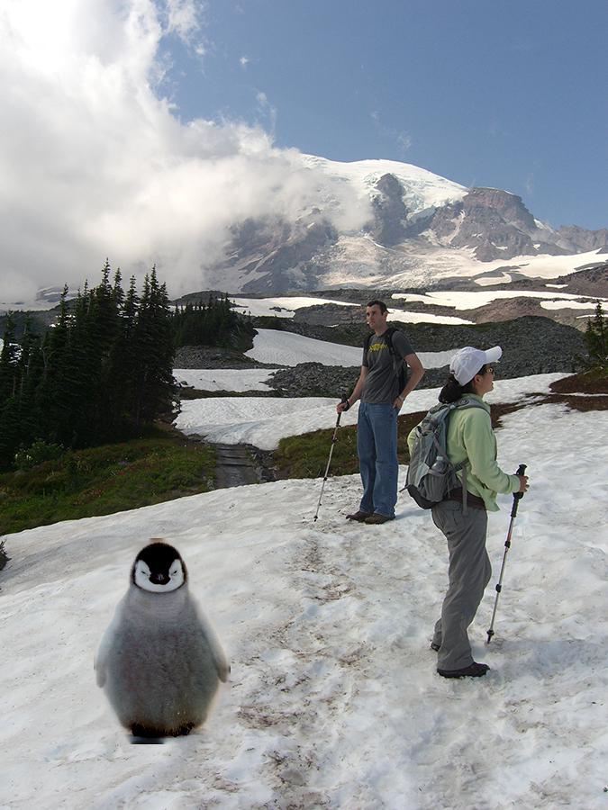
Blended
Dog on grass

Mask

Source

Target
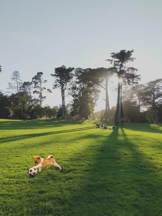
Blended
Tennis ball on concrete (failure case)
Possible failure explanations: the source image only has one RGB channel (green), the mask cropped too closely and
didn't leave any concrete around the ball.

Mask

Source

Target

Blended
Revisiting: Mooncake
Improvements: the background isn't blended to a medium gray, it stays white because we're directly copying pixels
from the target. Also it looks great in color! :)

Mask

Source

Target

Blended