Fun with Frequencies and Gradients

Frequency Domain Overview

The first part of this process explores manipulating images through the frequency domain. We see how 2D Gaussian blur filters can be used to split an image into different bands of frequencies. By isolating and combining frequencies, we can create effects such as hybrid images and perform multiresolution blending.

Warmup: Sharpen Filter

To create a sharpening effect, we try to emphasize the high frequencies of the image. We subtract the the image by a gaussian blurred version of the image to get the high frequencies and add it to the original image scaled by a factor to sharpen the image.

$sharpen(image) = image + \alpha(image - blur(image, gaussian(size, \Sigma)))$

To create a 2D gaussian kernel, two 1D multivariate normal distributions were multiplied together. To blur the image, we apply a FFT 2D convolution on the image using the kernel with symmetric padding.

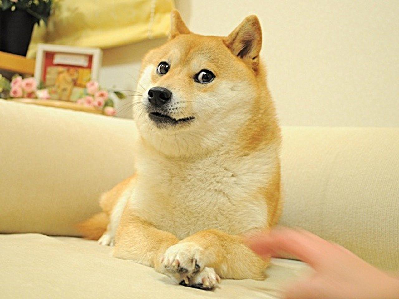
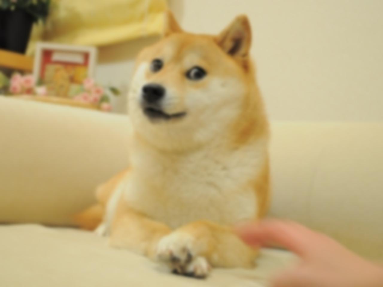
Crispy doge, $\alpha = 0.9, size = (37,37), \Sigma = 20$

doge.jpg	sharpen doge.jpg	blur doge.jpg

In the sharpened example above, the fur details on the doge is noticably crisper.

Hybrid Images

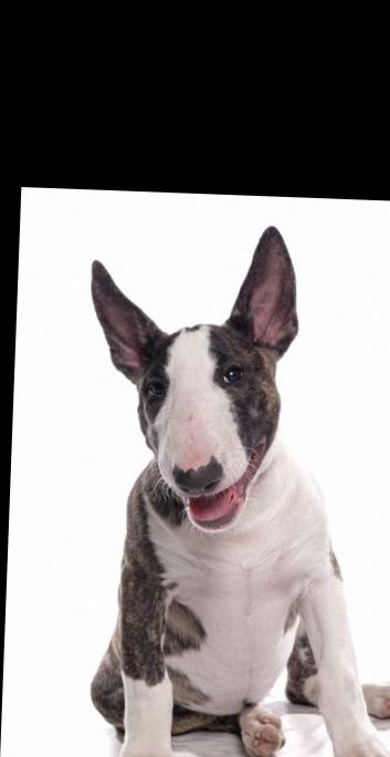
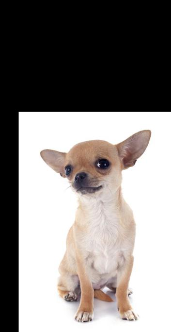
To create hybrid images, we follow the approach described by Oliva, Torralba, and Schyns in their 2006 SIGGRAPH paper. We combine the high frequencies of one image with the low frequencies of another to be able to see different images at different viewing distances.

$h(img_1, img_2) = \alpha_2(img_2 - b(img_2, g(size, \Sigma))) + \alpha_1b(img_1, g(size, \Sigma))$
where, $h=hybrid, b=blur, g=gaussian \ kernel$.

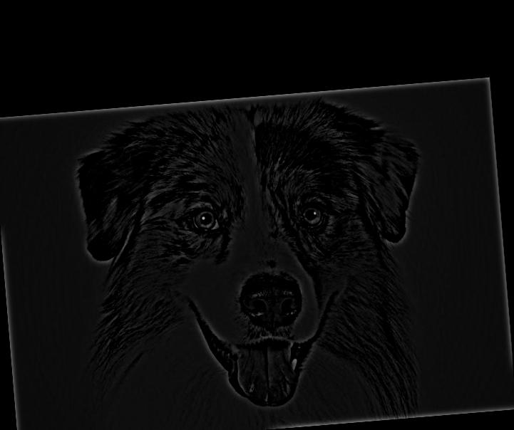
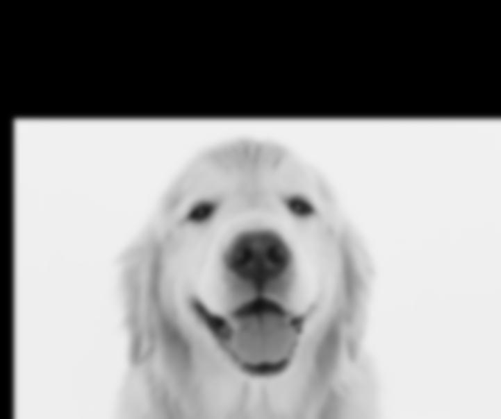
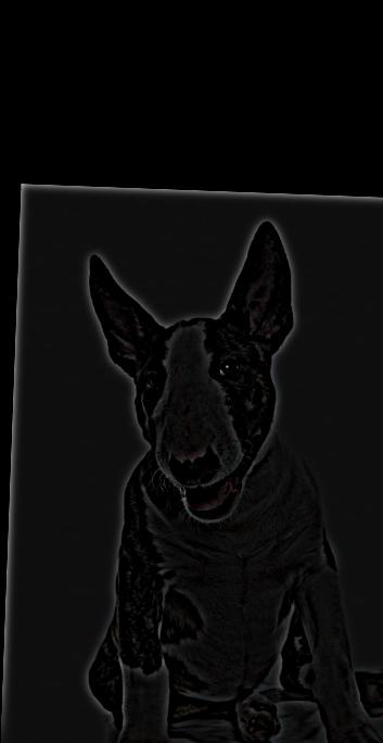
We first used the starter code to align two initial images by selecting two points on the first and second image that should correspond to each other. We then created the low frequency image by running image one through a 2D Gaussian filter. Inversely, the high frequency image two used the impulse filter minus the Gaussian filter: the original image subtracted by the Gaussian filtered version, like in the warmup. The two filtered images were then summed to create the final hybrid image.

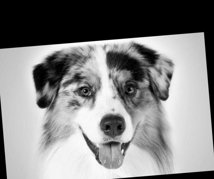
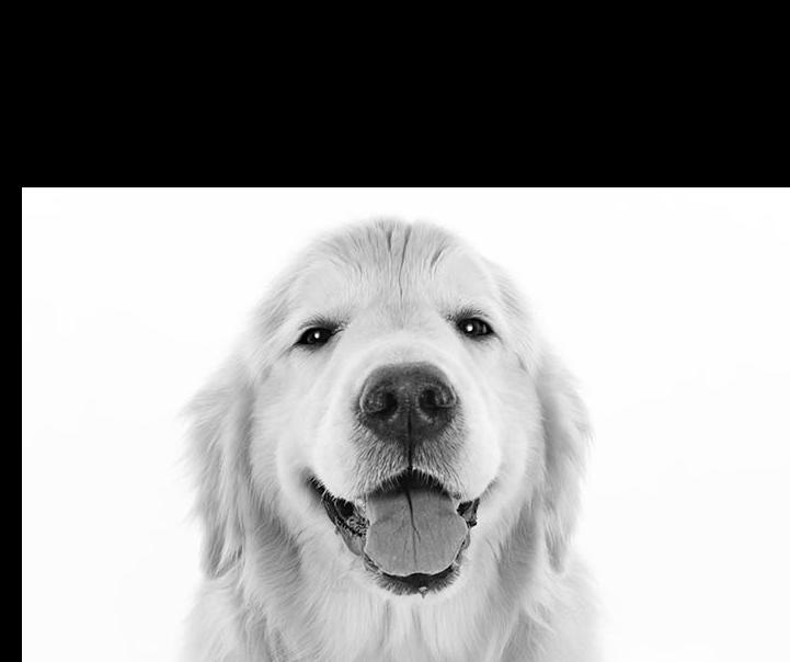
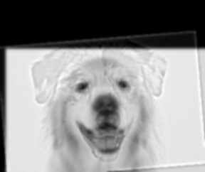
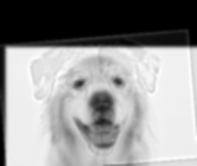
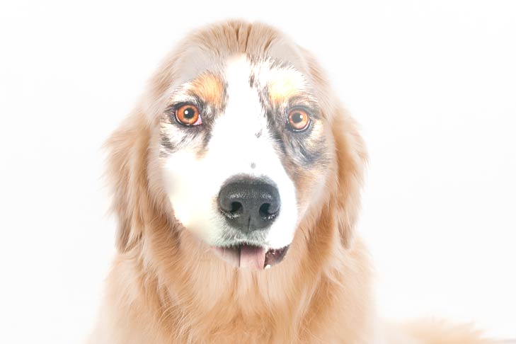
Golden collie, $\alpha_1 = 0.6,\ \alpha_2=0.5,\ size = (37,37),\ \Sigma = 17$

golden collie large	golden collie small

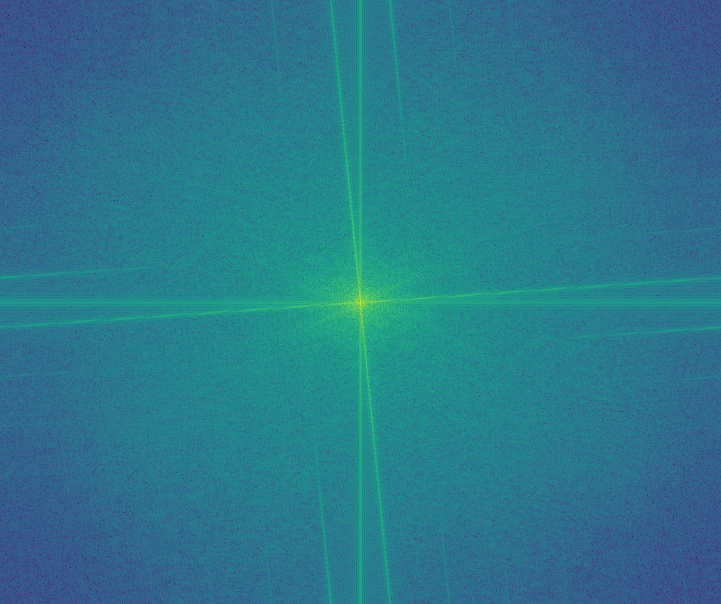
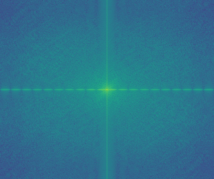
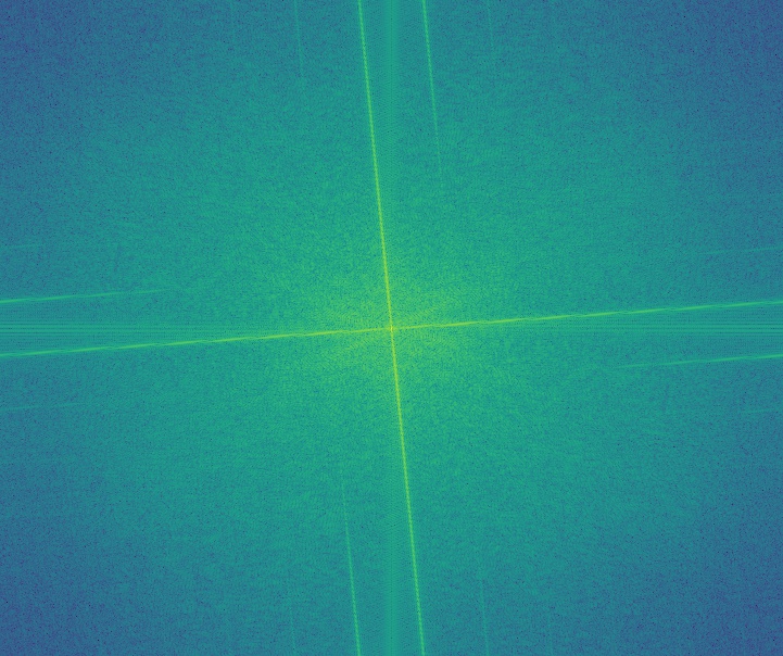
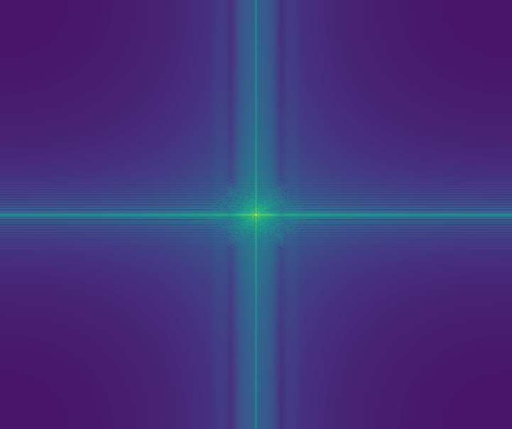
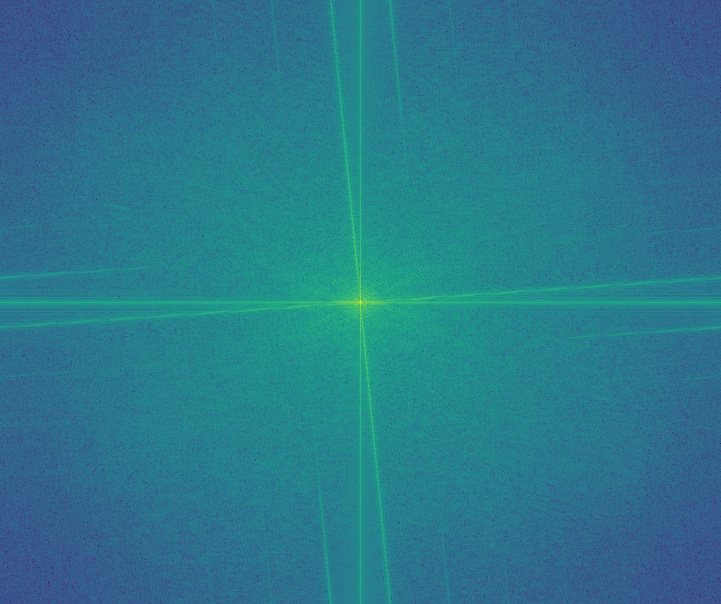
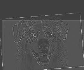
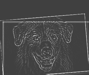
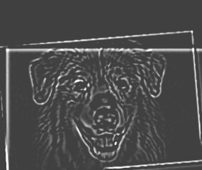
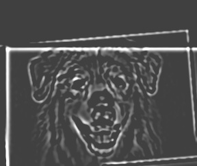
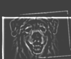
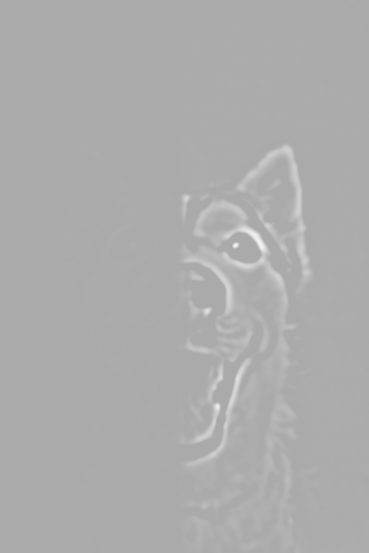
Golden collie frequency distribution

collie	retriever	high pass	low pass	hybrid

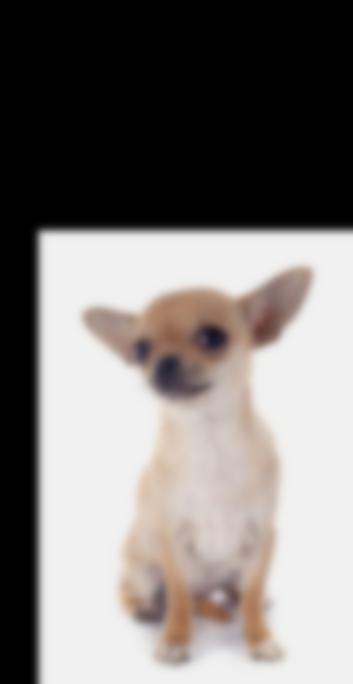
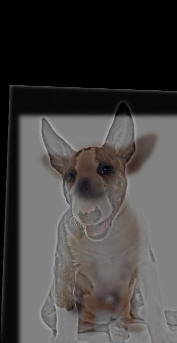
Ter-huahua silently judging

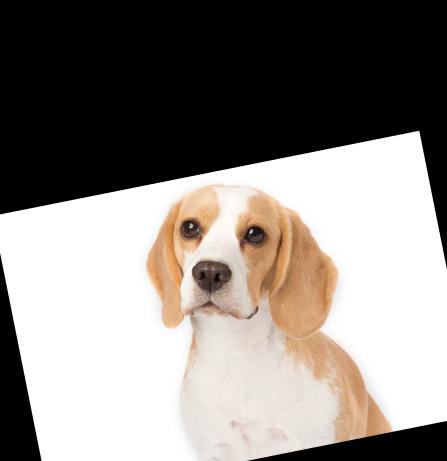
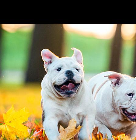
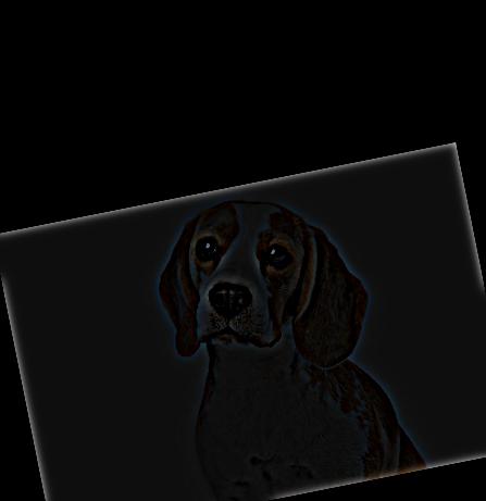
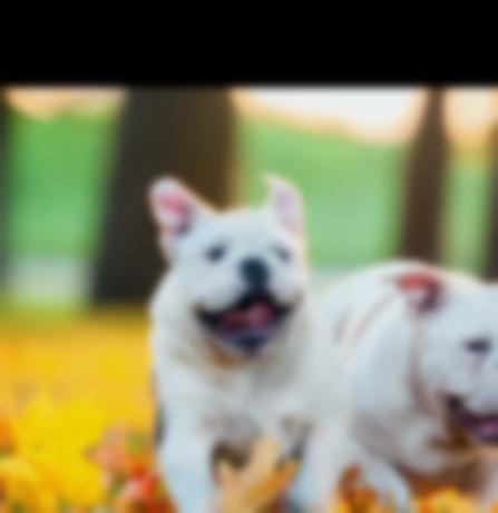
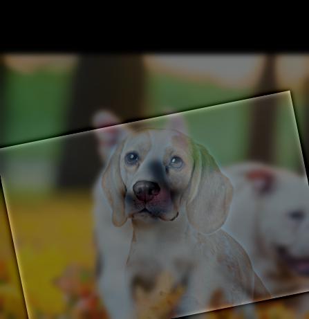
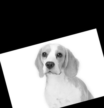
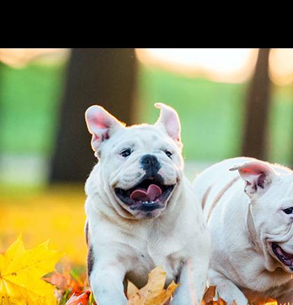
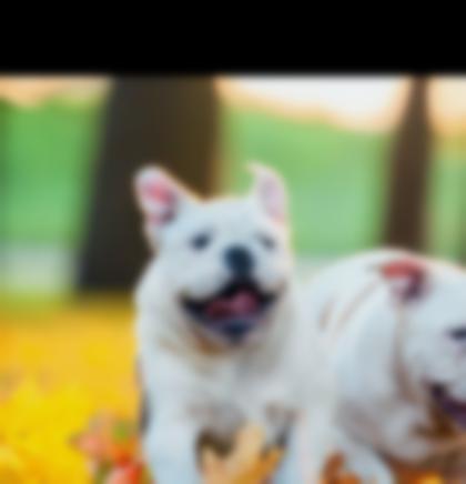
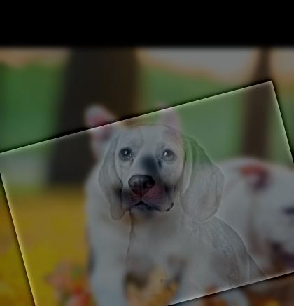
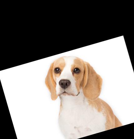
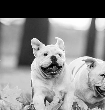
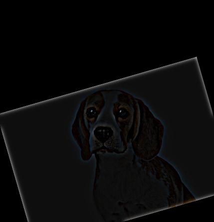
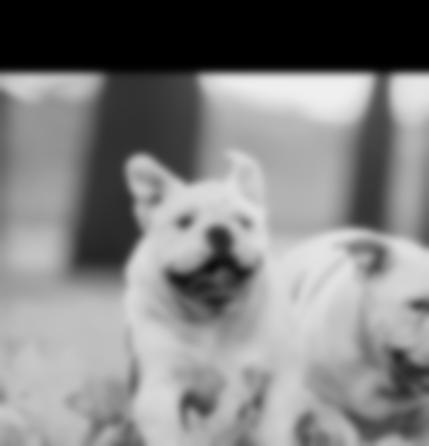
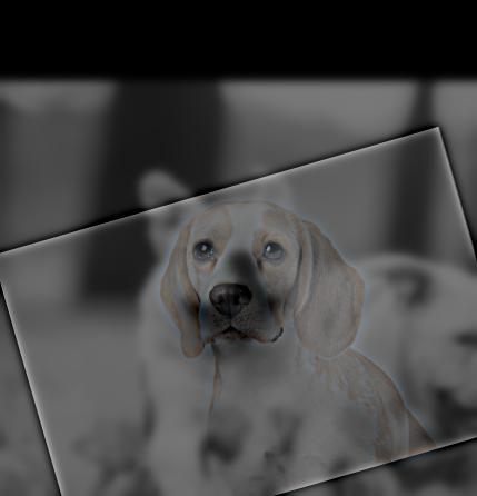
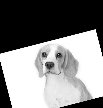
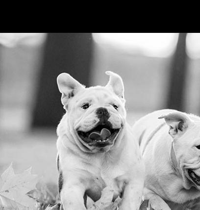
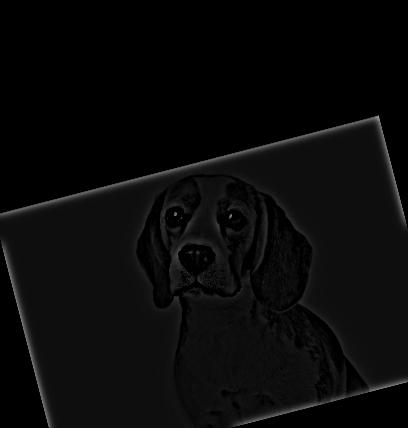
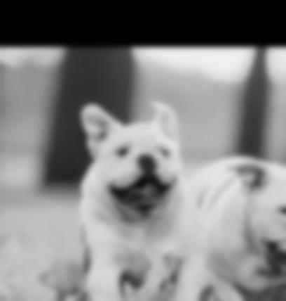
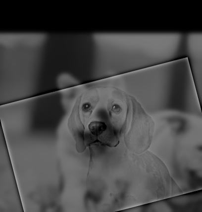
Beagledog?

This one doesn't look as good since the two dogs have entirely different poses and barely any overlap. We can also use this as an example to show the effect of color on hybrid images. As we can see, the high frequency image looks pretty similar regardless of color or greyscale. Meanwhile, the color enhances the low frequency image making the yellow leaves on the ground somewhat recognizable, while hard to distinguish on the greyscale version (for bells and whistles).

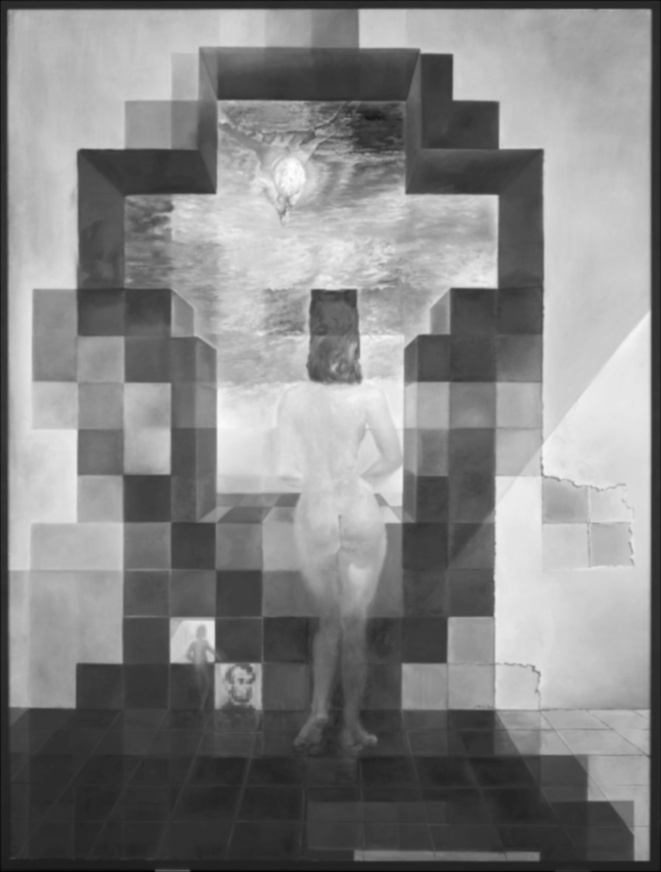
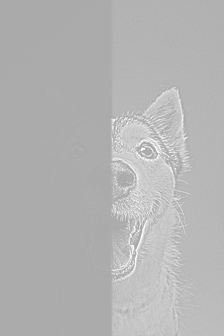
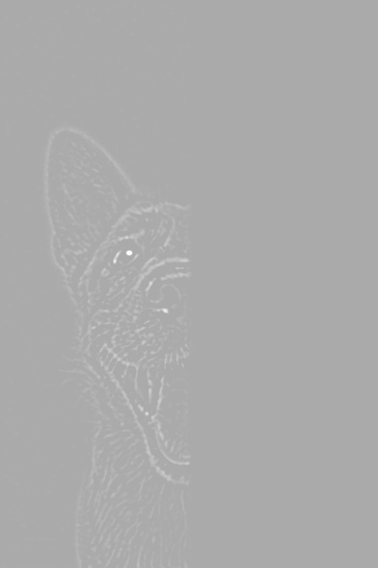
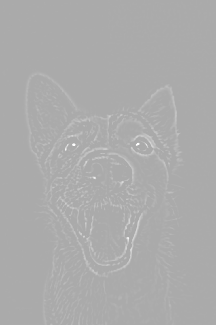
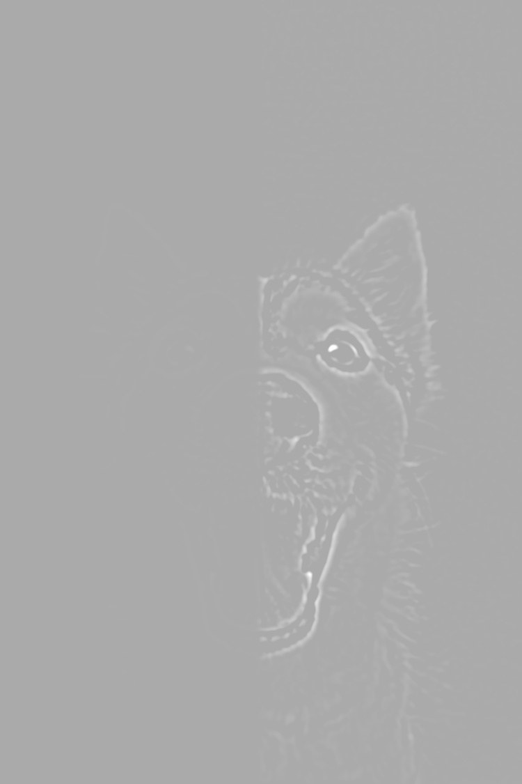
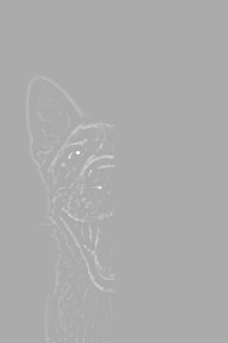
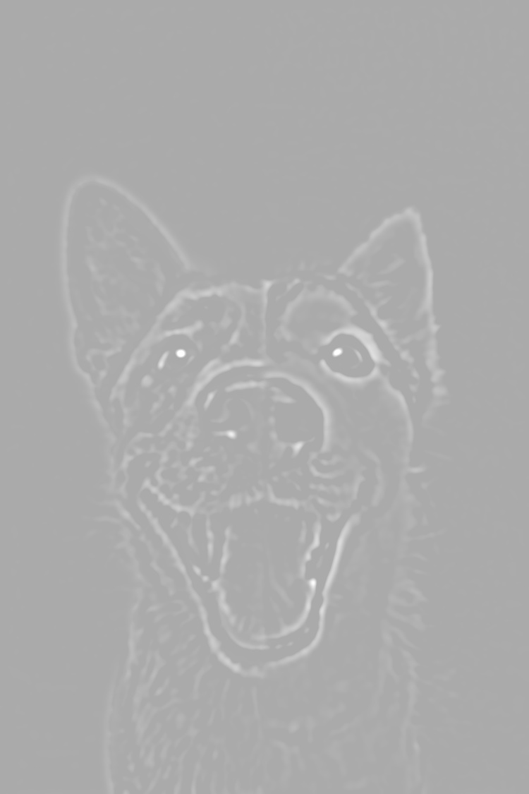
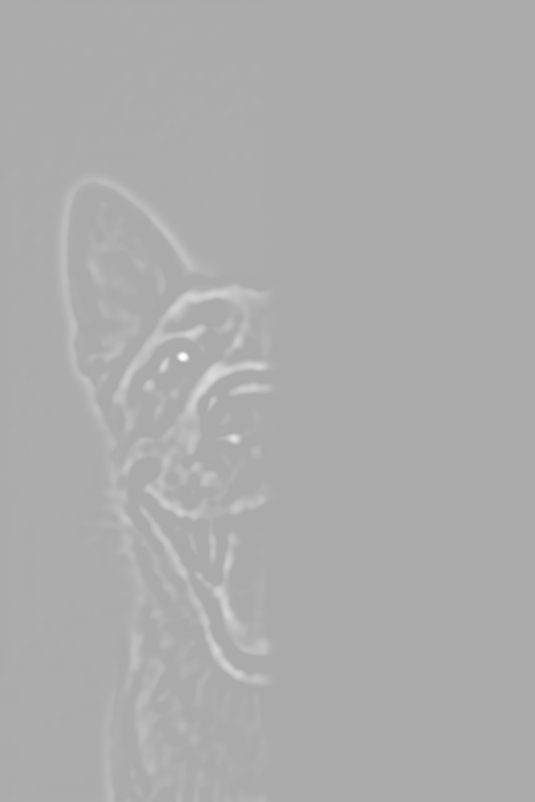
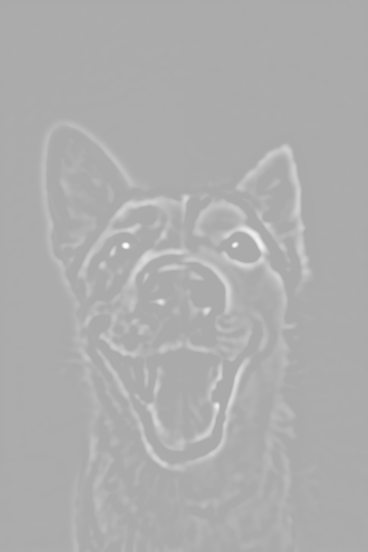
Gaussian and Laplacian Stacks

The Gaussian stack for an image is just a stack of the image filtered by Gaussian kernels of increasing intensity to split the image into different frequencies. The Laplacian stack is the difference in intensity between Gaussian stack layers, with each layer representing only the frequency at the specific band between Gaussian filtered frequencies.

In our implementation, we choose increasing powers of 2 to be our $\Sigma$ for successive layers in both stacks. The first layer in the Laplacian stack is the difference between the original image and the first layer in the Gaussian stack.

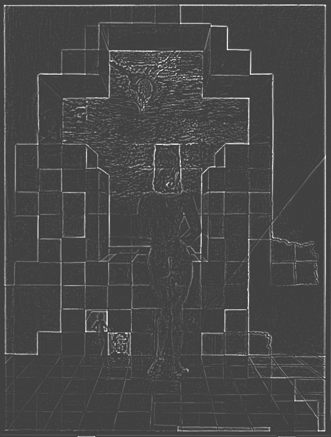
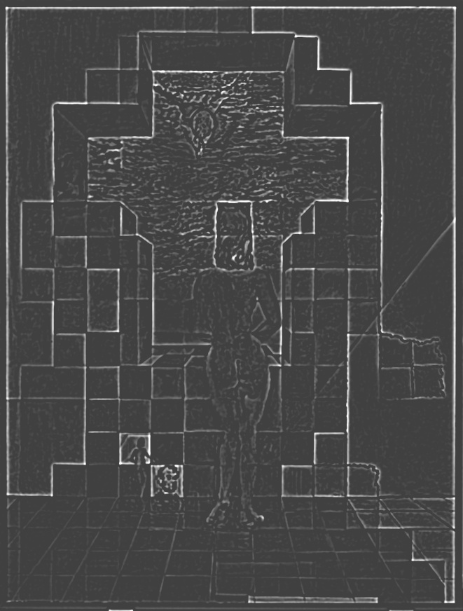
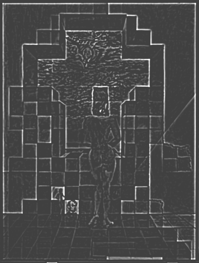
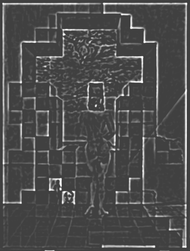
Gala Contemplating the Mediterranean Sea which at Twenty Meters Becomes the Portrait of Abraham Lincoln by Salvador Dali

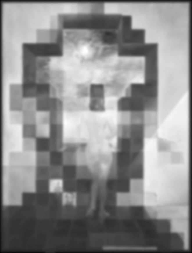
Gaussian stack
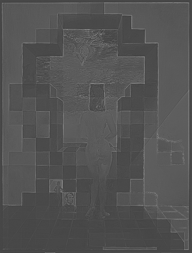
Laplacian stack
$\Sigma=1$	$\Sigma=2$	$\Sigma=4$	$\Sigma=8$	$\Sigma=16$

Golden Collie Redux

Gaussian stack
Laplacian stack
$\Sigma=1$	$\Sigma=2$	$\Sigma=4$	$\Sigma=8$	$\Sigma=16$

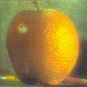
Multiresolution Blending

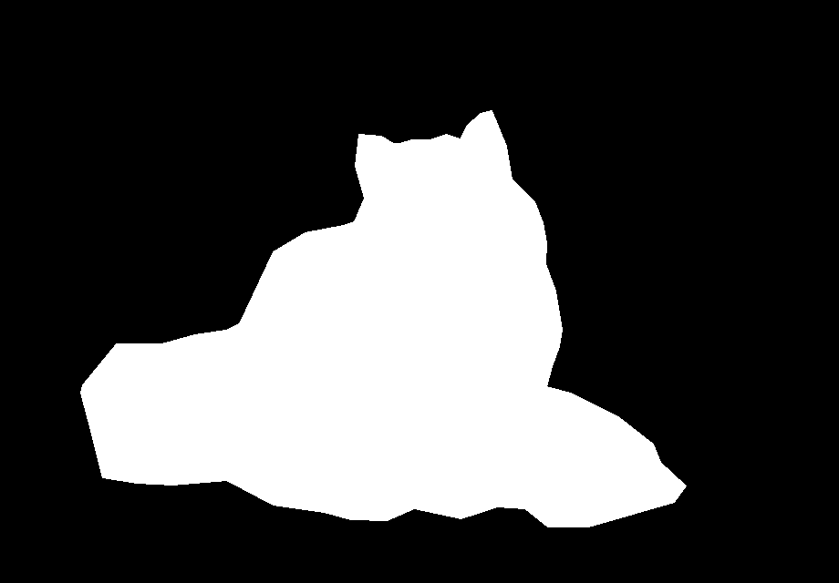
For multiresolution blending, we blend individual bands of frequencies in a pair of images by separately blending the layers of the laplacian stacks of two images. We first create a binary mask image that represents the boundary of where to blend. We then create a Gaussian stack for the mask image. Afterwards, we then blend individual layers of the Laplacian stacks for the two images using the corresponding mask Gaussian stack layer as the interpolation factor. Note: we have color blending (for bells and whistles).

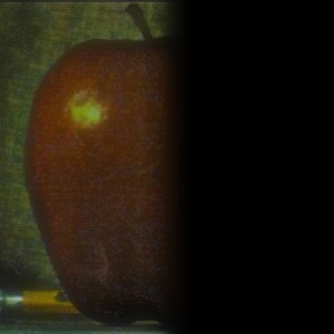
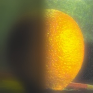
Orapple

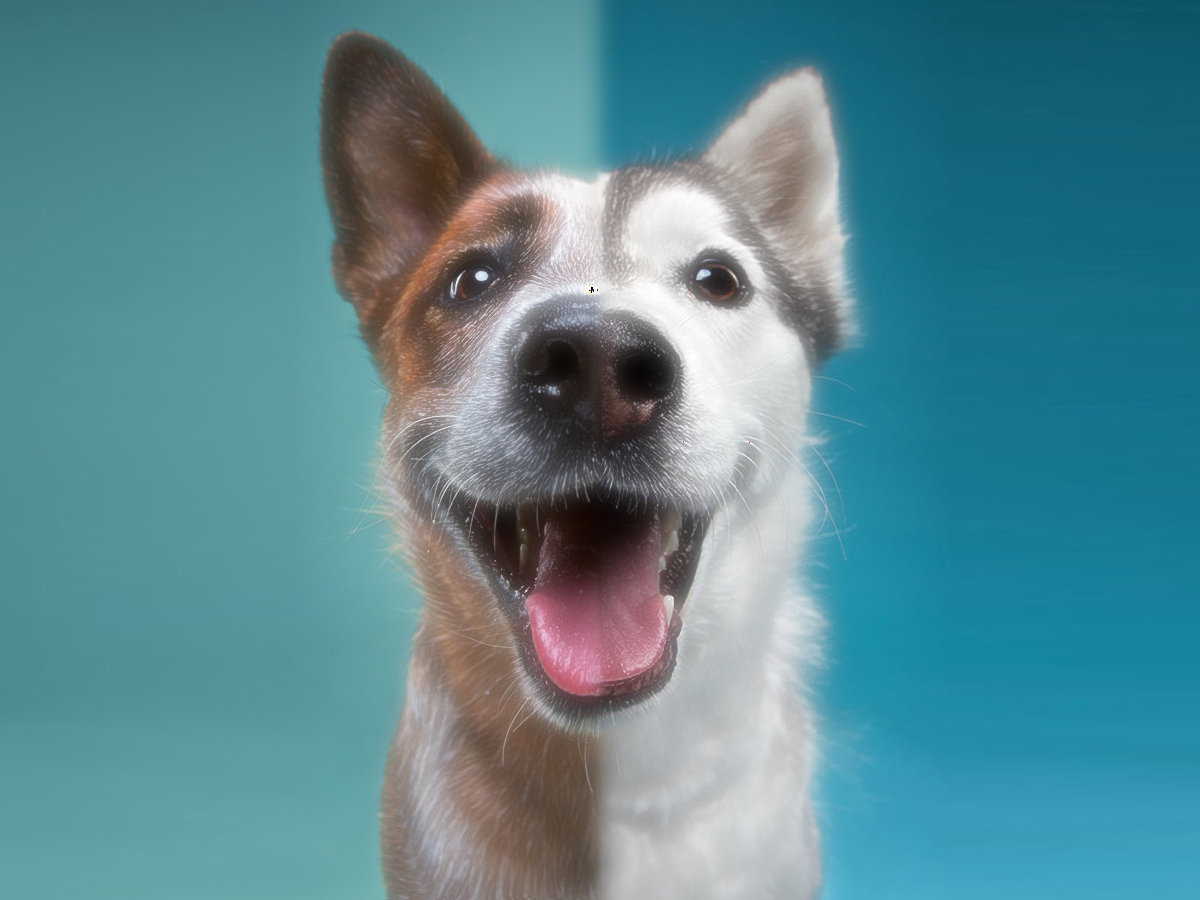
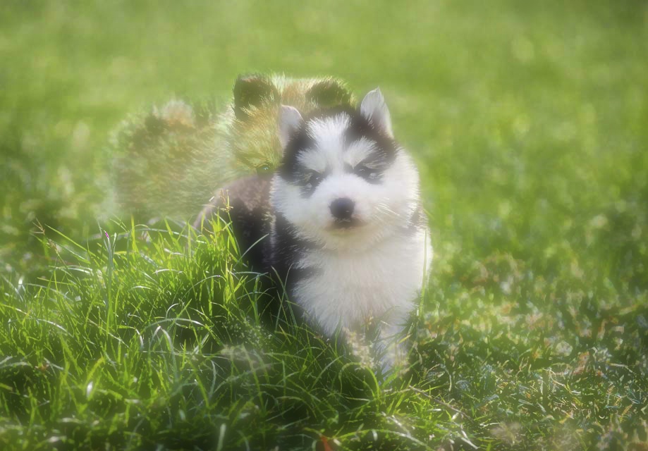
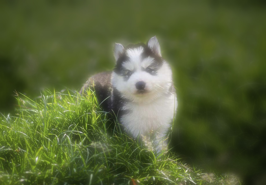
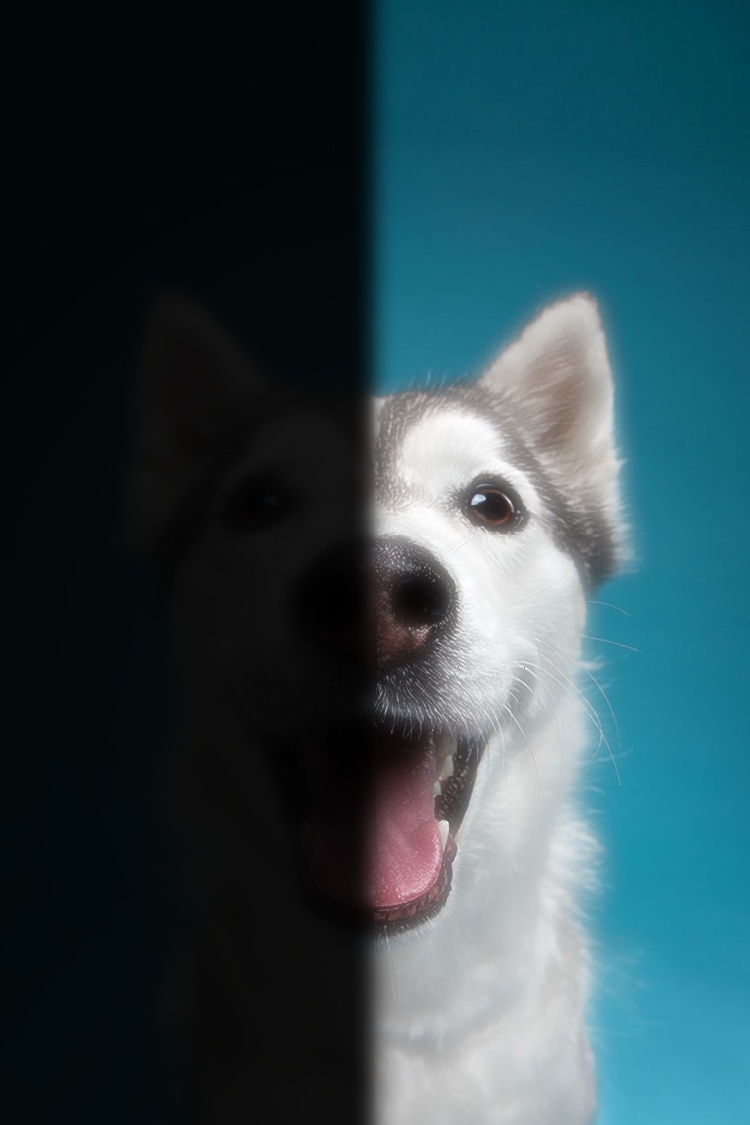
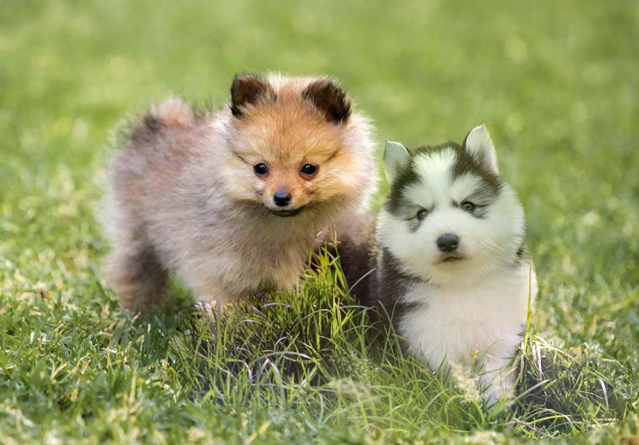
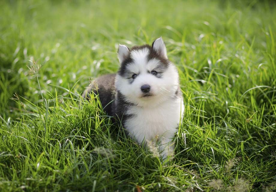
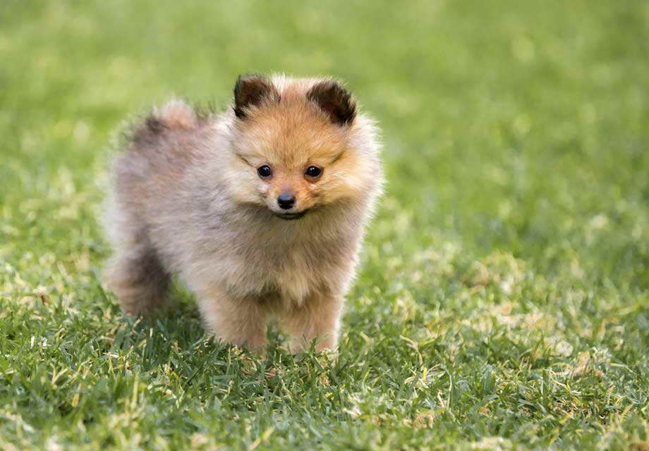
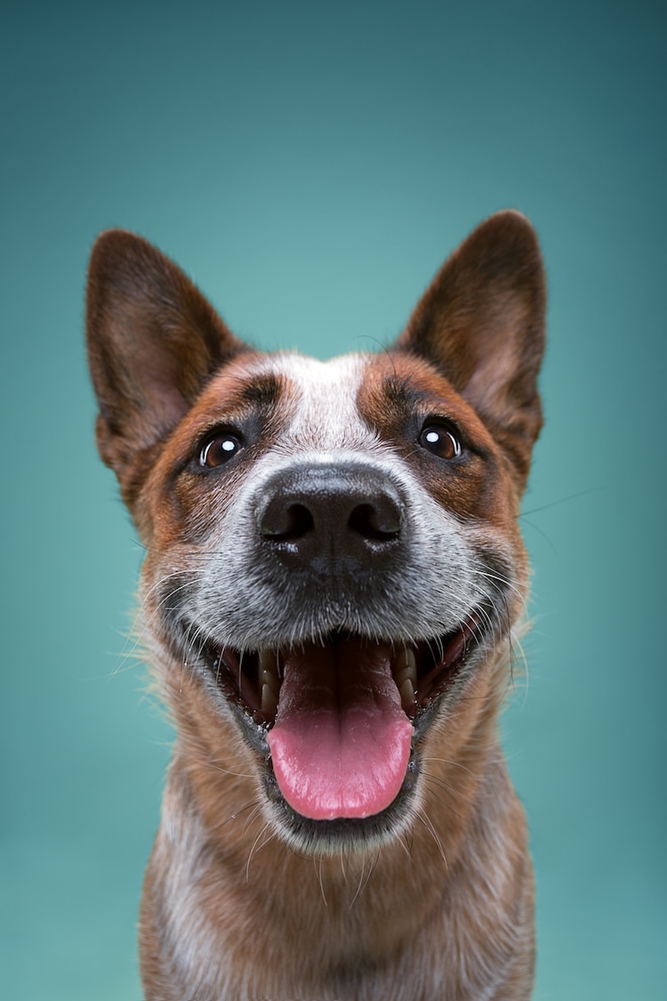
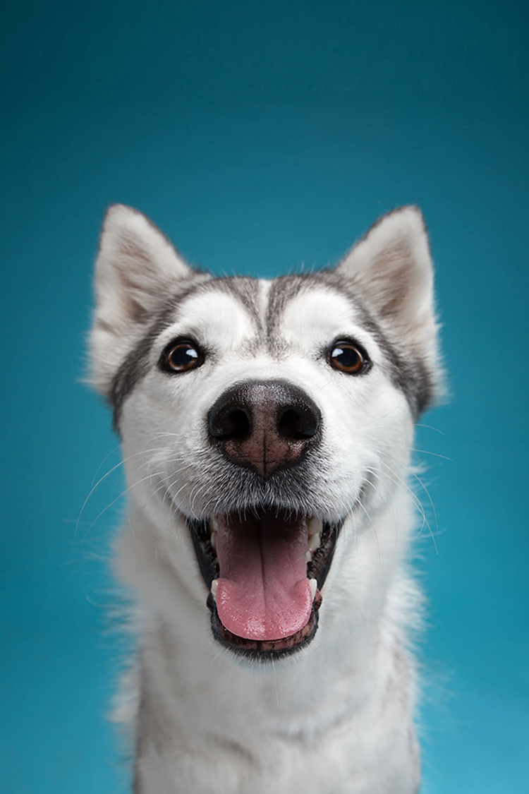
Husky and friend

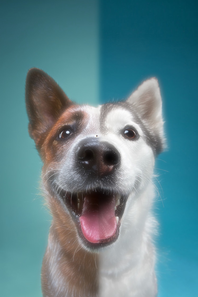
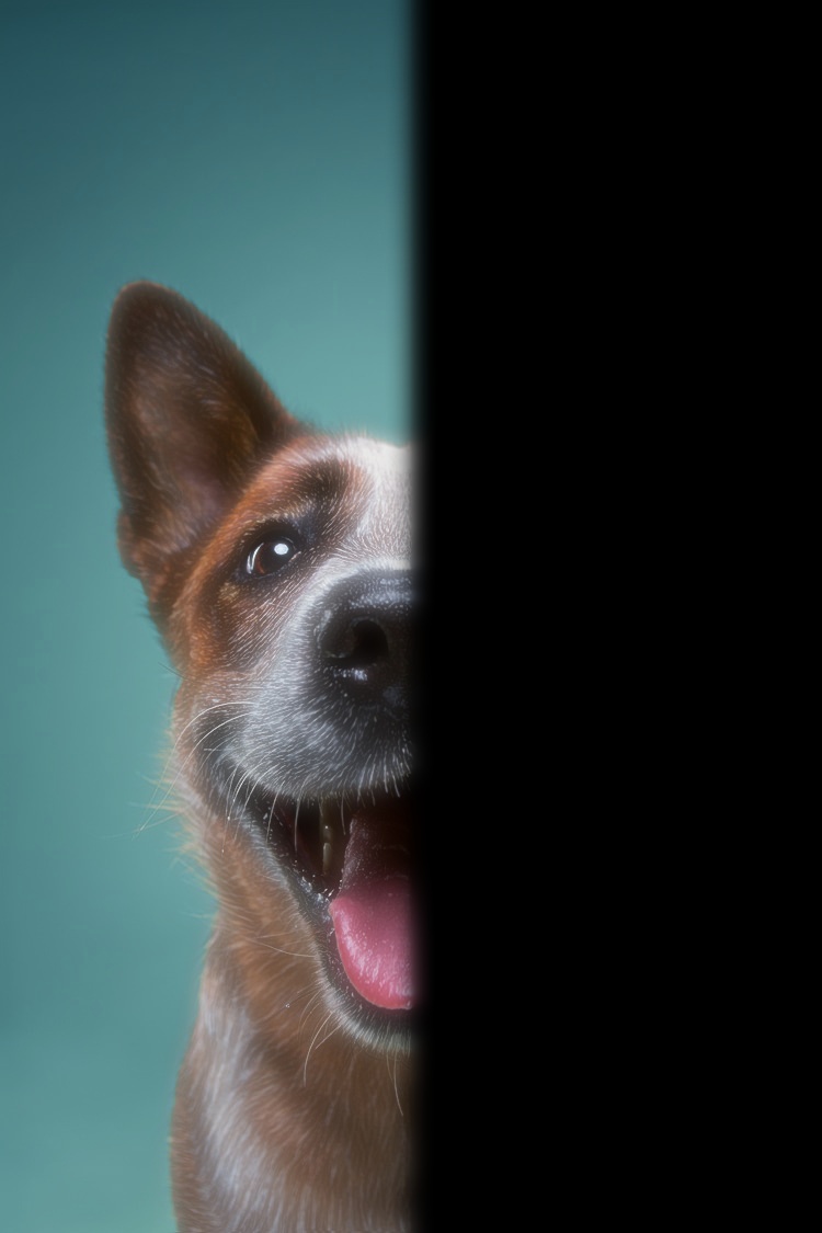
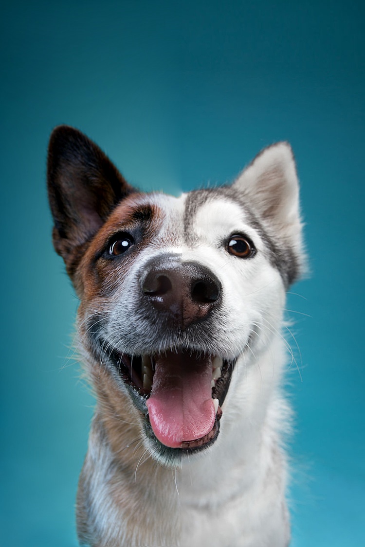
Good boy two face

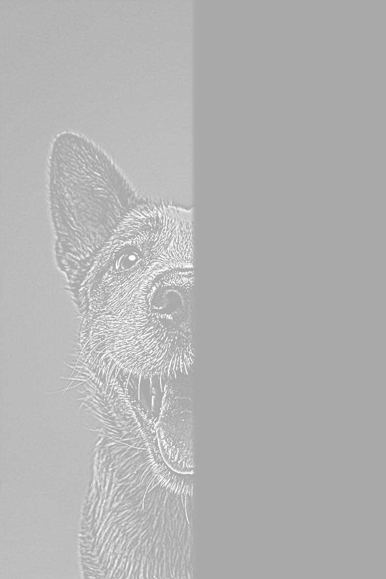
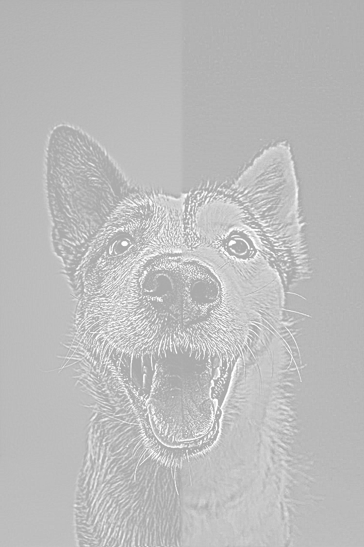
Two faced laplacian stack

Gradient Domain Overview

In this part of the project, we explore combine images on the gradient domain. In essense, we want to have the the pixels of the background image maintain their color while following the gradients of the source image. We choose to model this system as a constraint optimization problem through a method called Poisson blending.

In this equation, $i$ is a pixel in the source region $S$, and each $j$ is a 4-neighbor of $i$. We are trying to match the gradient of successive pixels in the target image to that of the source image region.

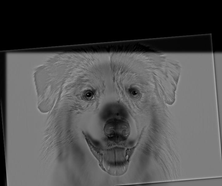
Toy Problem: Gradient Image Recovery

To start, the toy problem asks us to recover an image by the color of a single pixel and the gradient of the image. The warmup reduced to general Poisson blending with the constraint that the target/source area is the full image. We set up the Poisson blending constraints as a system of linear equations in the form of $Ax=b$.

$x$ represents the target pixel values we are trying to solve expressed as a column vector. In the toy scenario, each each element in $x$ is a pixel value we are looking for.

$A$ is a sparse matrix where each row represents gradient and hard constraints that the target pixels need to be optimized. For the toy warmup, there are two different types of constraints expressed in the rows. First, the coefficient in the row corresponding to the $x$ pixel value we have needs to be set to 1. Afterwards, for the gradient constraints, the row coefficients corresponding to $(x, y)$ and $(x, y + 1)$ are set to -1 and 1 respectively for every $(x, y)$ combination. This corresponds to the vertical gradients. The same must be done for $(x, y)$ and $(x+1, y)$ for the horizontal gradients.

$b$ is a column vector with equal entries as rows in $A$, representing the resulting constants from each linear equation constraint. This represents the actual gradient difference corresponding to each $A$ row.

Once $A$ and $b$ were filled in using the original image, we can run the equation through a sparse linear solver, scipy.sparse.linalg.lsqr , to get the resulting $x$ pixels.

Original	Reconstructed

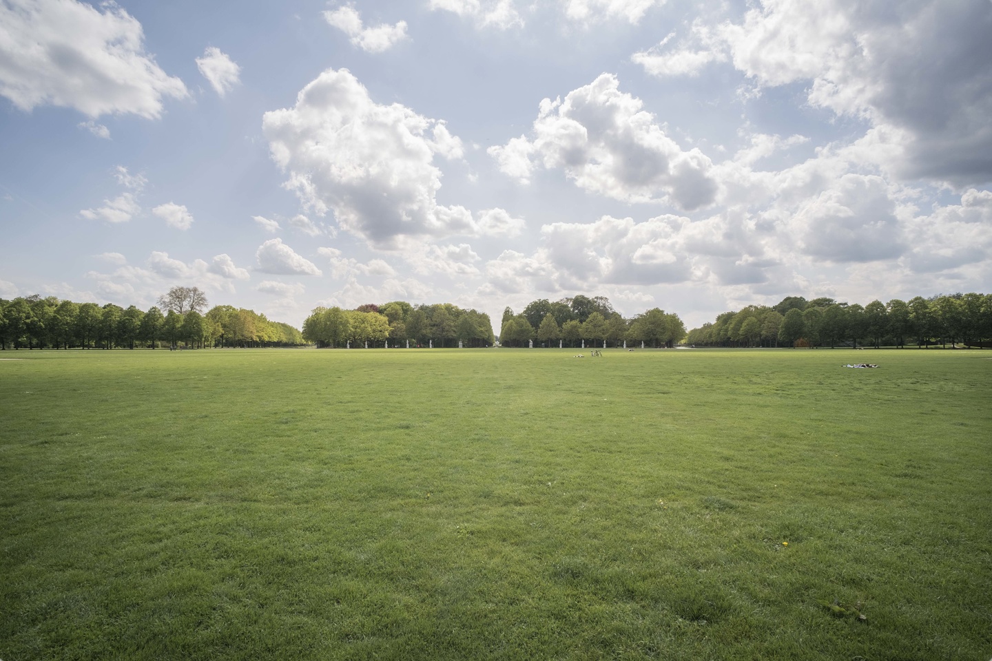
Poisson Blending

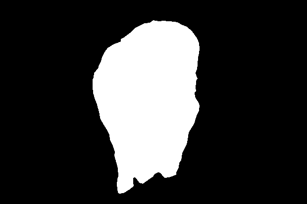
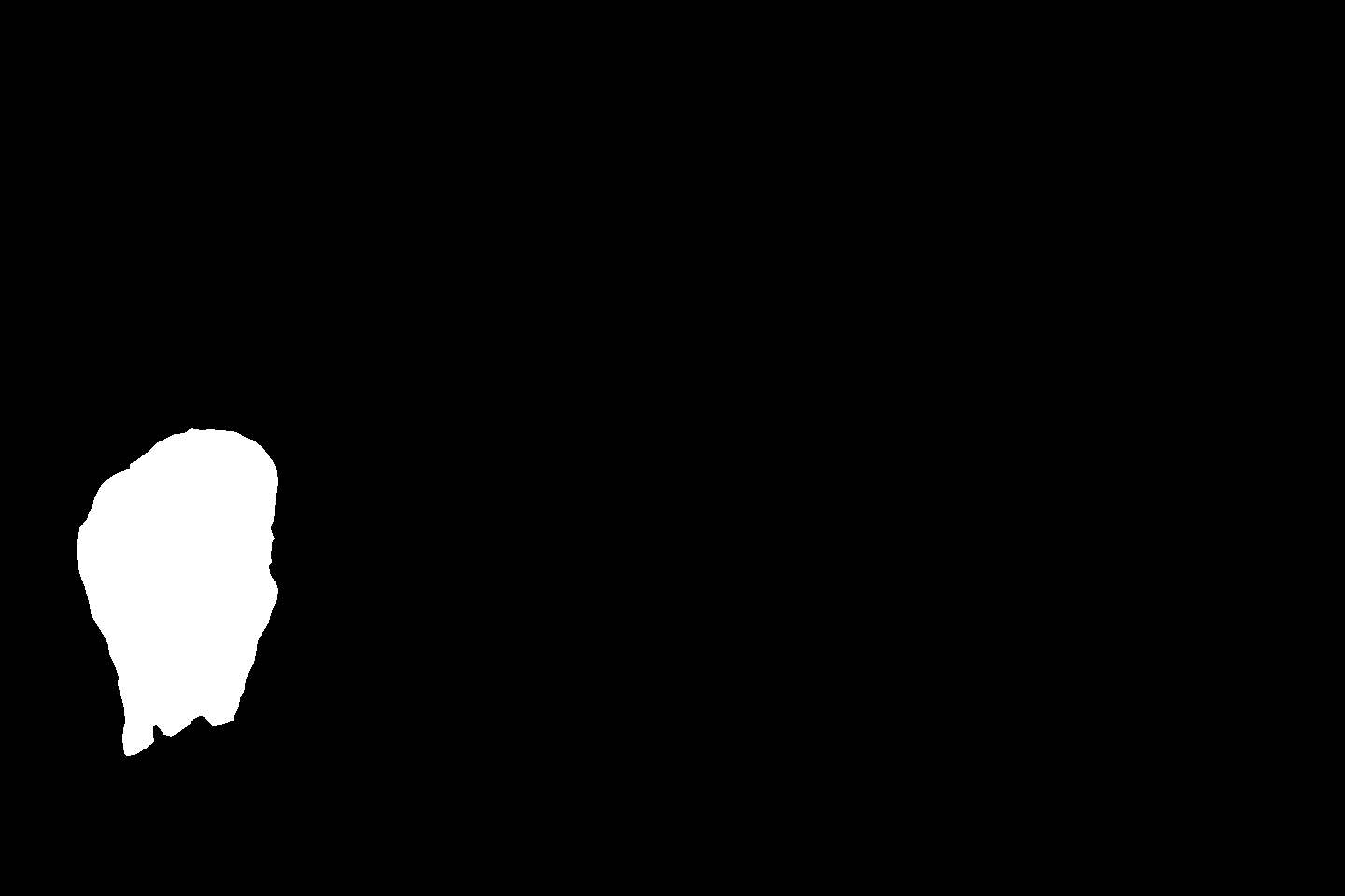
For general case Poisson blending, we use a binary mask with the same masked shape for both the target/source images to know which pixels from the source should map to the target. Once we know the corresponding pixels in the image, we can generate $A$ and $b$ to forms the rows of the constraint. The difference between the general case and the toy is that the entire boundary of the masked shape must take the value of the target image. Therefore, instead of having a single hard pixel intensity constraint, we have many. Our implementation maps these intensity constraints to the inner border with the mask shape. Afterwards, a sparse linear solver was used again to find the best solution. Finally, we map the found pixel intensities onto the target image.

Also thanks to Nikhil Uday Shinde for his starter code to generate binary mask images.

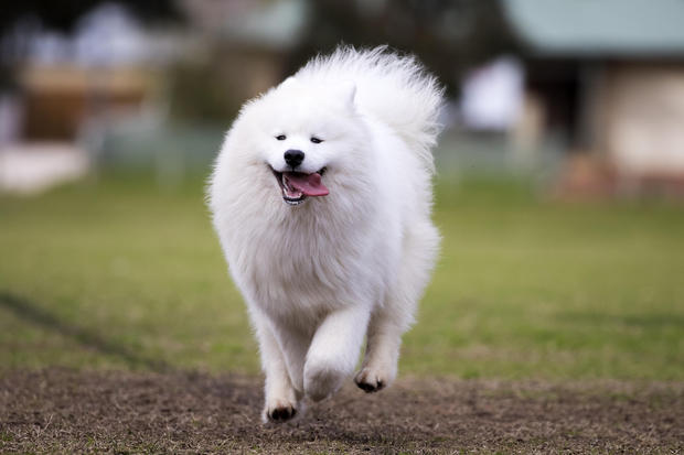
The real golden collie

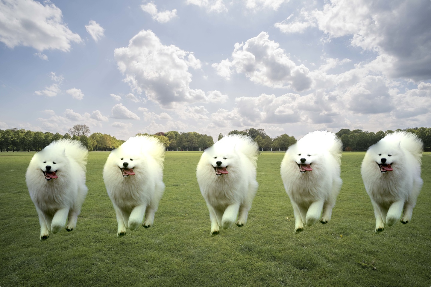
Squad up

Husky and friend redux

The above image is an example that did not turn out so well. We can see that the top of the husky's head starts to turn green due to the the green of the background. Of course this could have been remedied by expanding the mask a little around the husky so the gradeints start from the green background in the source image. In addition, the bottom right of the blended image shows a noticable seam. This is due to the suden change in frequencies between the low frequency target image and the high frequency source.

Two faced Laplacian/Poisson comparison

Laplacian	Poisson

We use the same split mask as in Poisson blending as in the Laplacian blending. We see that Poisson blending has left the full background of the blended image in a more consistent color and maintained a lot of sharpness in the image. The separation boundary is a lot more sharp in certain parts of the dog such as the nose and the tongue, but is seamless for most of the fur. The Laplacian image is much softer in the blending boundary, and has a slight blur because I turned up the Gaussian intensity pretty high. We see that Laplacian work well if the original colors need to be preserved. However, if the source and target have similar textures, Poisson works really well to create seamless transitions without losing any frequency information.

In this specific case, we think Poisson blending works a lot better. The background and fur blending without resolution loss makes it seem much more like a single image, despite certain hard boundaries at the nose and tongue.