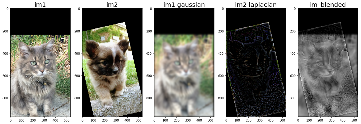
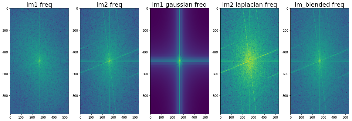
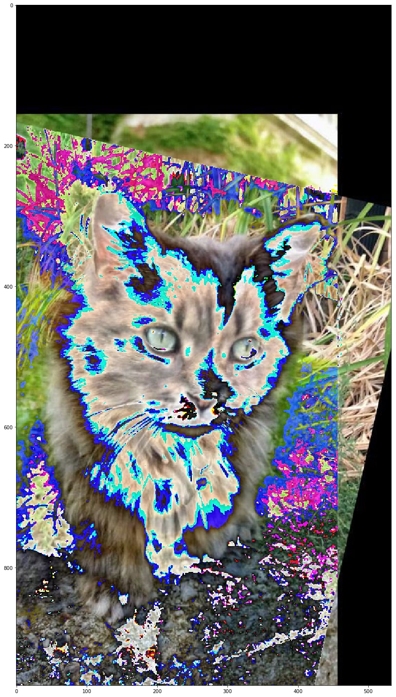
A qualms with this image is that the dog and cat look very similar so some of their features or not as distinguishable. However, I really liked this hybrid since you can really see from the gaussian and laplacian stacks the two separate images.
In class, we learned about different ways to transform and morph images based off of their frequencies. First, we covered the idea of a gaussian, which when convolved with a source image acts as a low pass filter. In essence, the gaussian will blur the image and remove high frequencies from the source. On the flip side, the laplacian is the opposite, a high pass filter. The laplacian can be calculated as the source image minus the gaussian, which leaves you with edges/high frequencies. We are using various frequency and gradient analysis to "photoshop" our own images!
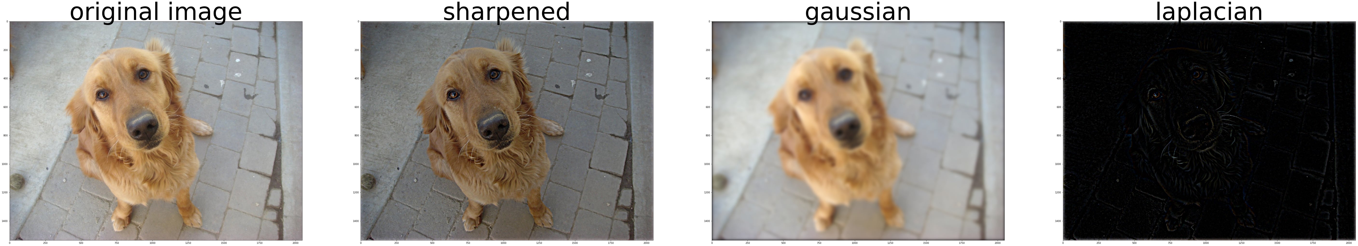
For this portion, I picked a blurry-ish image and sharpened it. The math behind this process is to take the gaussian of the image (blurred portion) and subtract it from the original to get the laplacian (edges of the image). From here, you can add the laplacian (high frequencies) back to the original image to emphasize the existing edges.
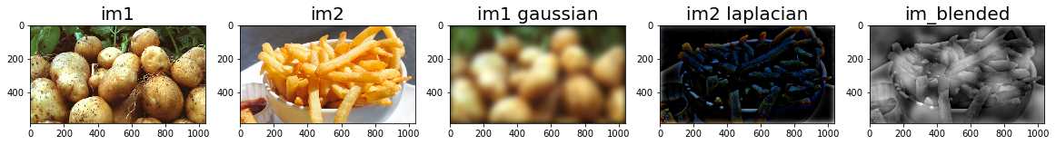
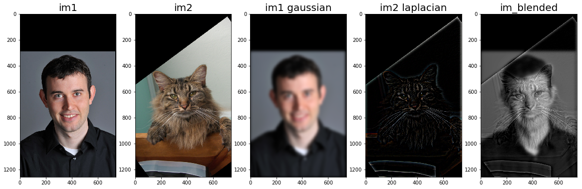
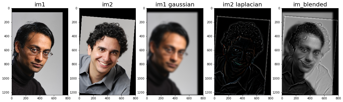
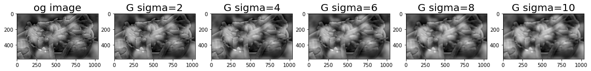
The goal of this section was to take two images and create a hybrid one by summing the gaussian of one and the laplacian of the other. My process for finding this was first aligning the images on features then finding the best sigma by iterating through various values until I found one visually appealing.
catski = pomski + cat
A qualms with this image is that the dog and cat look very similar so some of their features or not as distinguishable. However, I really liked this hybrid since you can really see from the gaussian and laplacian stacks the two separate images.
potatoes = fries + potatoes
derecat = Derek + Nutmeg
Failures: ee16a = sahai + maharbiz
In my opinion, this blending was a bit of a failure since there are discrete changes in the image color. Thus, the laplacian does not overlay as nicely and subtly over the gaussian. Another reason for failure was that I could not find a suitable sigma such that when you applied the gaussian/laplacian stack, Sahai and Maharbiz were visible. With a larger sigma, after applying the gaussian over the image, you could still clearly see Maharbiz's face when in fact, we just want to see that of Sahai. However, with a smaller sigma, you are not able to clearly see Maharbiz's face.
Failures: Wrong image type
I also encountered a failure with images not adding correctly even after clipping. I found that my images were uint8 and was able to fix the problem when I converted them to type float64.
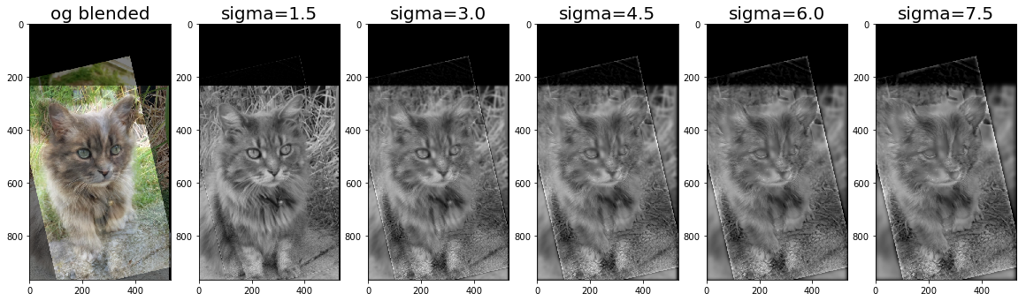
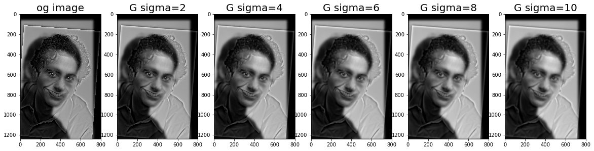
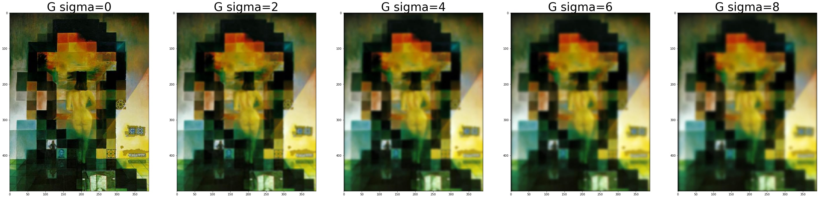
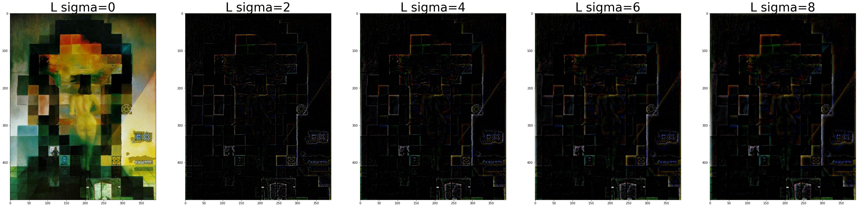
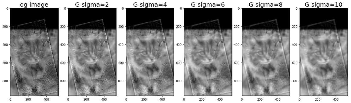
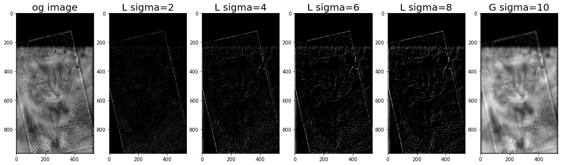
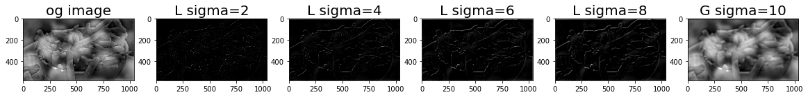
The goal of this section was to take an image and create an optimized gaussian/laplacian stack using the prior image in the stack. This helps to reduce computation time since convolving with larger and larger gaussians is more work compared to iteratively applying teh same gaussian to an image or image that already had a gaussian applied. The laplacian stack was created such that the summation of all images in the stack will yield the original. Thus, the last image in the stack will be the final gaussian. You can tell from the following images that with the gaussian stack, you can see more and more of the blurred image while in the laplacian stack, you can see more and more of the edges of the sharper image. The equation is set up as such
Lincoln Lady
Catski
Potatoes
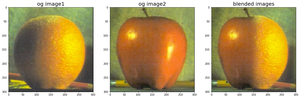
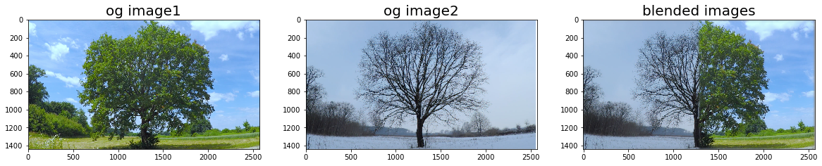
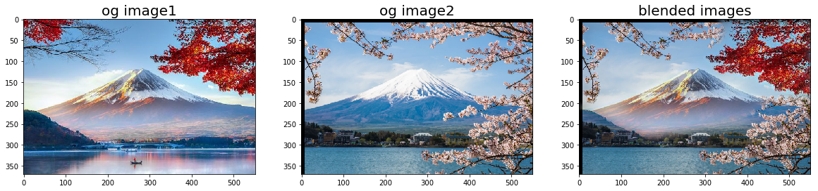
In the section, we stitch two images together by blending both on various frequency bands. This is done by first creating a binary mask, then applying our gaussian/laplacian stack on the source, target, and mask images. We then apply the equation below to blend individual levels of each stack.
Results!
Failure! 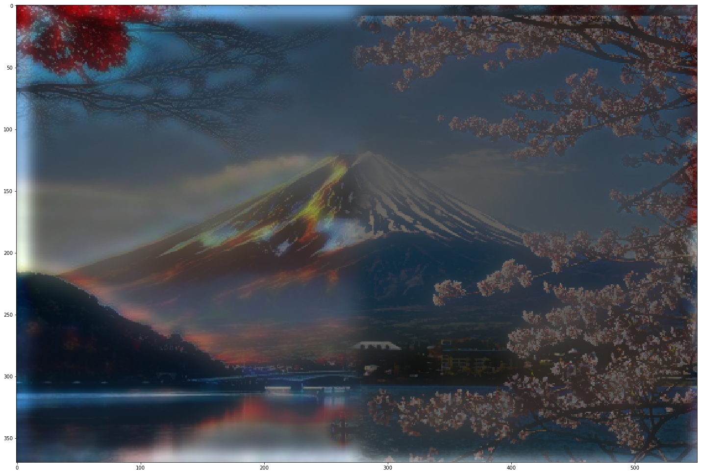
Thus far, most of our analysis of images has been in terms of pixel intensities (0,255) or in the frequency domain (gaussian/laplacian). Another way to represent an image is in terms of the gradient. This is very useful especially in the realm of blending since you can also maintain pixel intensity in addition to the frequency details of the image. In this second part, we will explore utilizing gradient domain to better blend our images together by maintaining the gradient within the source but maintaining the pixel intensities of the target.
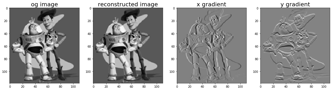
In this section, our goal is to reconstruct the toy.jpg image using constraint optimization (in the form of Least Squares). We construct a sparse (1's and -1's) matrix A which represents the gradient and have it equate b, the calculated gradient of our toy image. Additionally, to maintain the pixel intensity, since the gradient does not store any that information, we add an aditional constraint that the top left pixel value should remain the same intensity as what it was originally. Then, we apply least squares on our sparse matrix (A) and gradient image (b) to try to reconstruct the original image (v). This section was a good preliminary part to help us reconstruct the original image from an x,y gradient vector. Note, I say vector because we flatten the 2d image into a 1d vector.
Results!
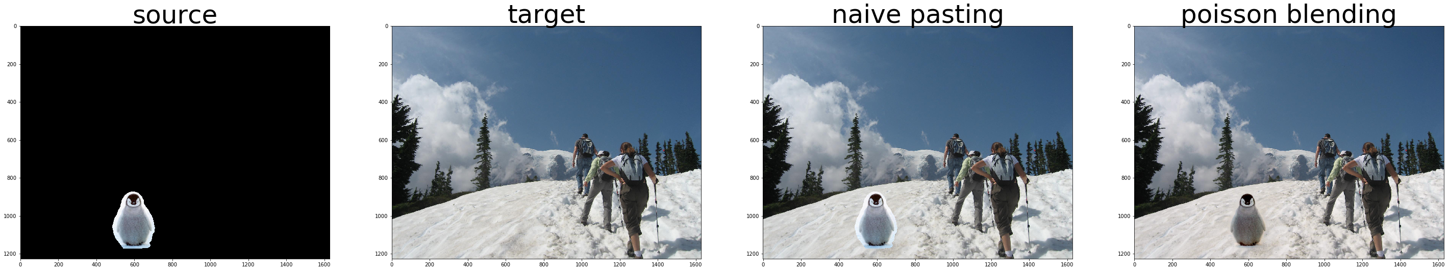
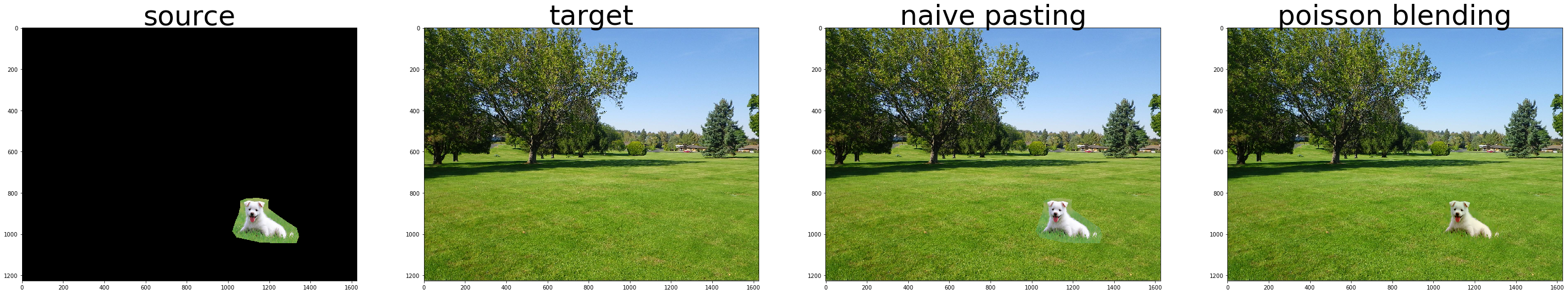
For this final section, we apply least squares onto another constraint optimization problem. In this case, we construct a new gradient and A sparse matrix to match the idea of retaining a target's gradient but also retaining the source's pixel intensity. The left side of the following equation ensures that the gradient inside the mask but not on the boundary of the mask is the same as the gradient in the source image. Meanwhile, the right side of the following equation ensures that the pixel value on the border is the same as that in the target. Thus, we are able to set the color of the borders of the new image and let the gradients determine what hte pixel value should be.
Instead of using the intended equation above, I merged the x gradient and y gradient system of equations in to one large equation that encompases both. Thus, I was able to reduce my sparse matrix's (A) size to just be n x n where n equals the number of pixels in the mask of the image. The equation I used is as follows... The left side reprsents the new image (V) and its gradient with the target (T) while the right side is the gradient of the source image (S). Note, for the left side, T will be utilized instead of V for any pixel location that is not in the mask so the utilization of V and T will vary.
Results!
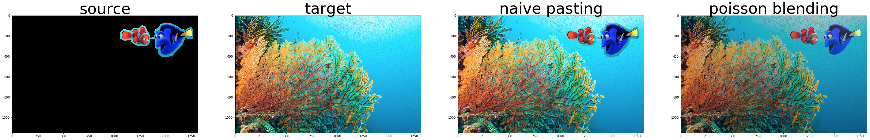
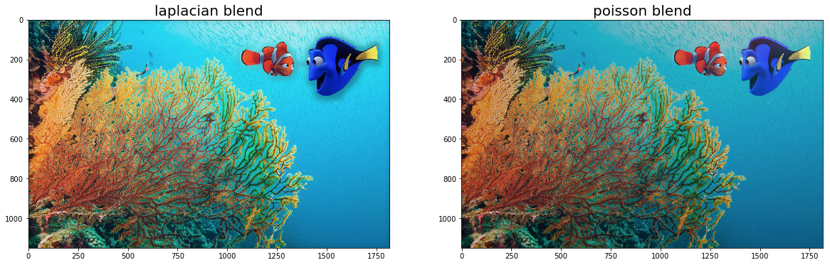
I found the nemo picture to be quite peculiar since the image after poisson blending was net darker. However, I used the same algorithm on all of my poisson blendings and no other image had a dark artifact. This was very odd but overall, the blending was still pretty nice. This may be because the color intensity pixel was chosen from inside the mask. However, I implemented the same algorithm to all pictures and only this one was an abnormality. So I cannot quite attest to what went wrong.
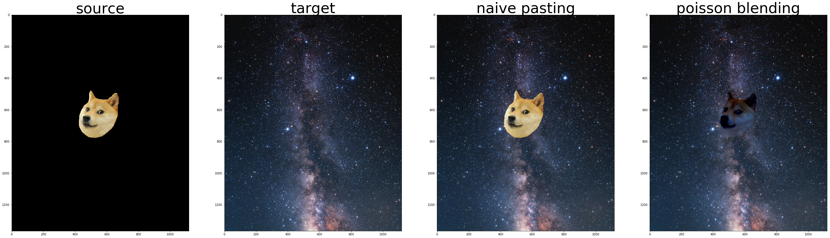
Failure: I found the doge galaxy image to be a use case failure since the doge adopted the color of the background and turned purple. Aside from that, everything worked out pretty well.
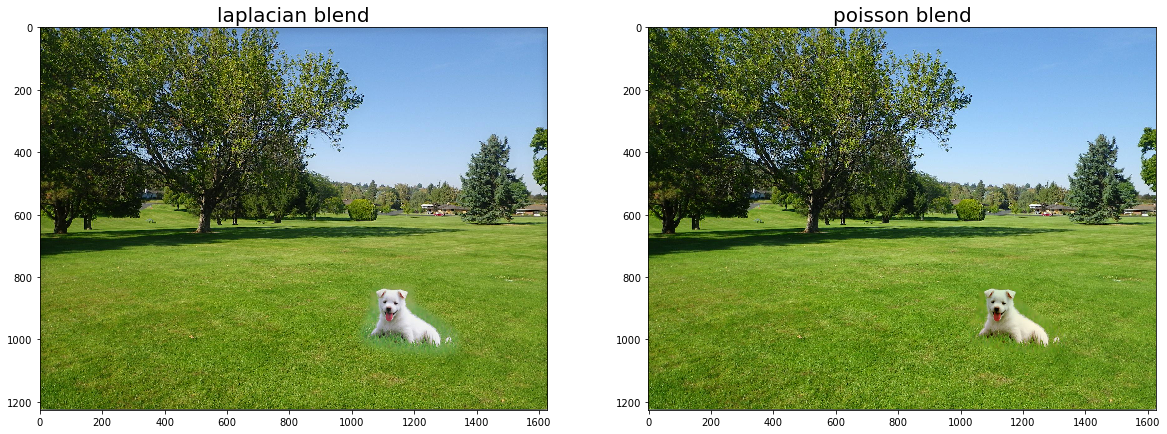
Laplacian vs Poisson
The comparison between the laplacian and poisson blending shows how laplacian only blends edges whereas poisson blends edges by trying to reduce the gradient and maintaining color intensity.