Fun with Frequencies and Gradients!

CS194-26: Computational Photography Fall 2018

Clarence Lam, `cs194-26-abh`

Part 1.1: Sharpening

Unsharp Masking Filter

The unsharp masking filter actually sharpens images, by adding "detail" to the original image. This "detail" is obtained by subtracting a blurred version of the original image from the original image, which in effect results in a high-pass version of the original image. This "detail", high pass filtered image contains the edges of the image. We finally add this "detail" to the original image to make the edges sharper.

$\text{im}_{\text{sharp}} = \text{im}_\text{og} + \alpha(\text{im}_\text{og} - \text{im}_\text{blur})$

Instead of using scikit-image's built in gaussian blur function, I wrote a simple function to convolve the image with a 2D gaussian kernel, with kernel length and sigma as adjustable parameters. As default, I used a $ 11 \times 11 $ Gaussian kernel with $ \sigma = 9 $. The after photos below the original photos used $ \alpha = 0.5 $.

Part 1.2: Hybrid Images

Overview

Hybrid images are static images that change in interpretation as a function of the viewing distance. The basic idea is that high frequency tends to dominate perception when it is available, but, at a distance, only the low frequency (smooth) part of the signal can be seen. By blending the high frequency portion of one image with the low-frequency portion of another, you get a hybrid image that leads to different interpretations at different distances.

Implementation

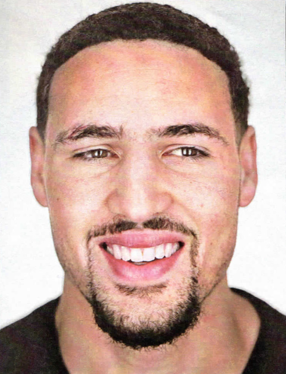
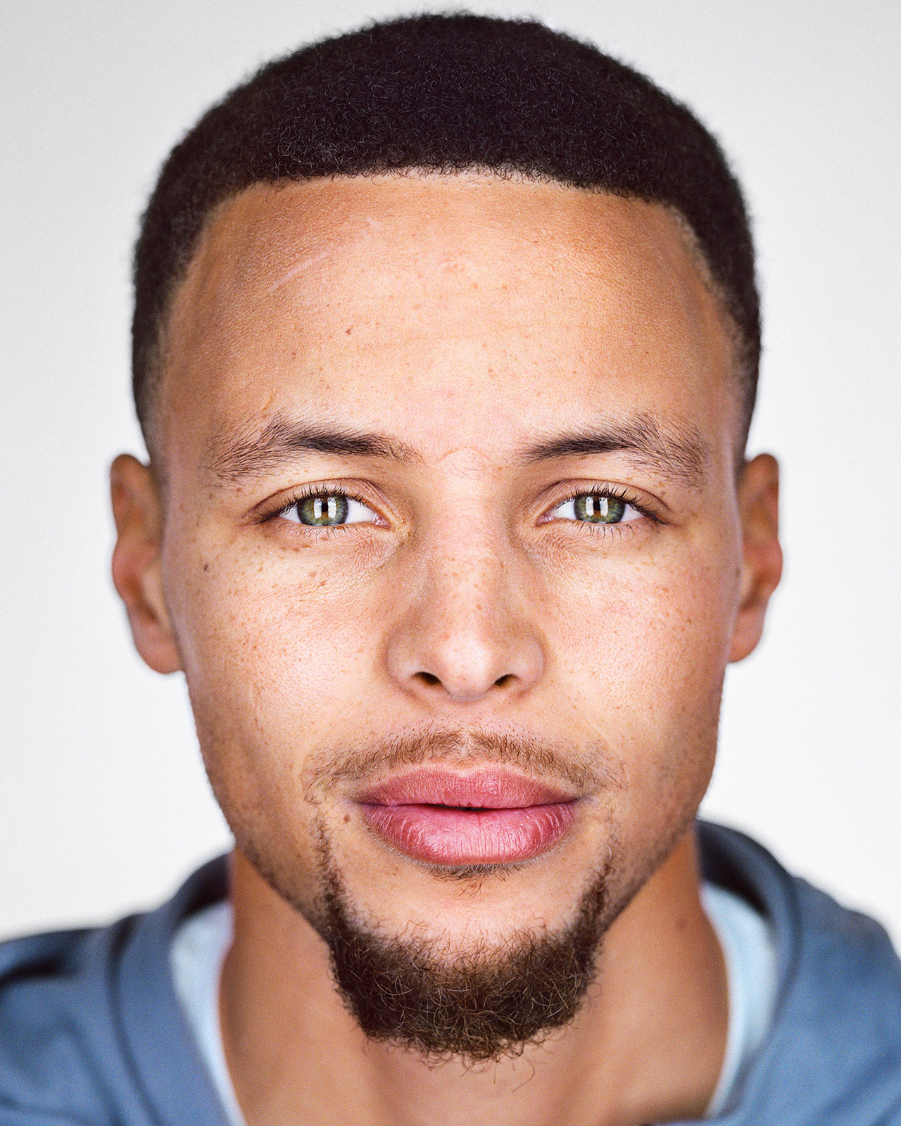
First things first was to find pairs of images that could be overlaid onto each other, with features that could be intuitively and visually aligned, such as eyes; this alignment is important because it affects perceptual grouping.

Next, I used my aforementioned gaussian blur function to low-pass filter one image, and the unsharp masking filter from part 1.1 to high-pass filter the other.

Finally, I averaged the two images, with alpha weights for the two images that summed to one. I kept color in both the low-pass and high-pass images and thought the results looked good (Bells and Whistles). Here are some of my favorites; one way to simulate viewing at different distances is to zoom in or zoom out the images / this page.

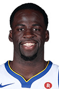
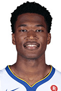
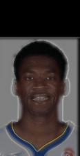
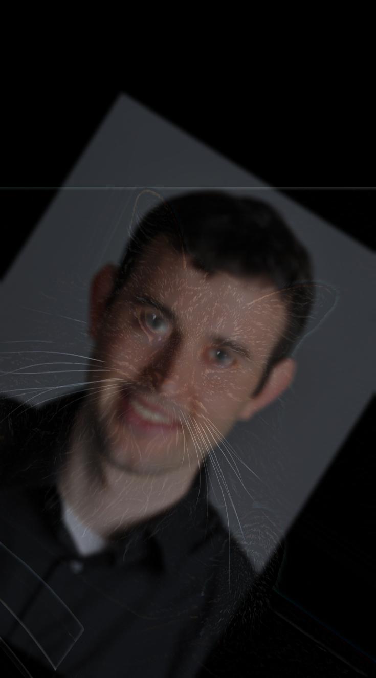
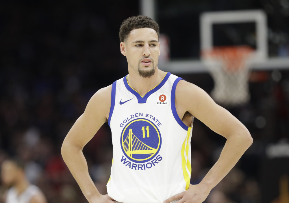
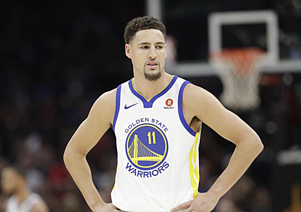
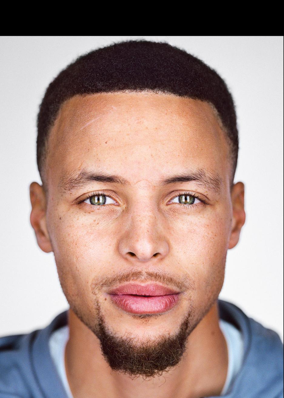
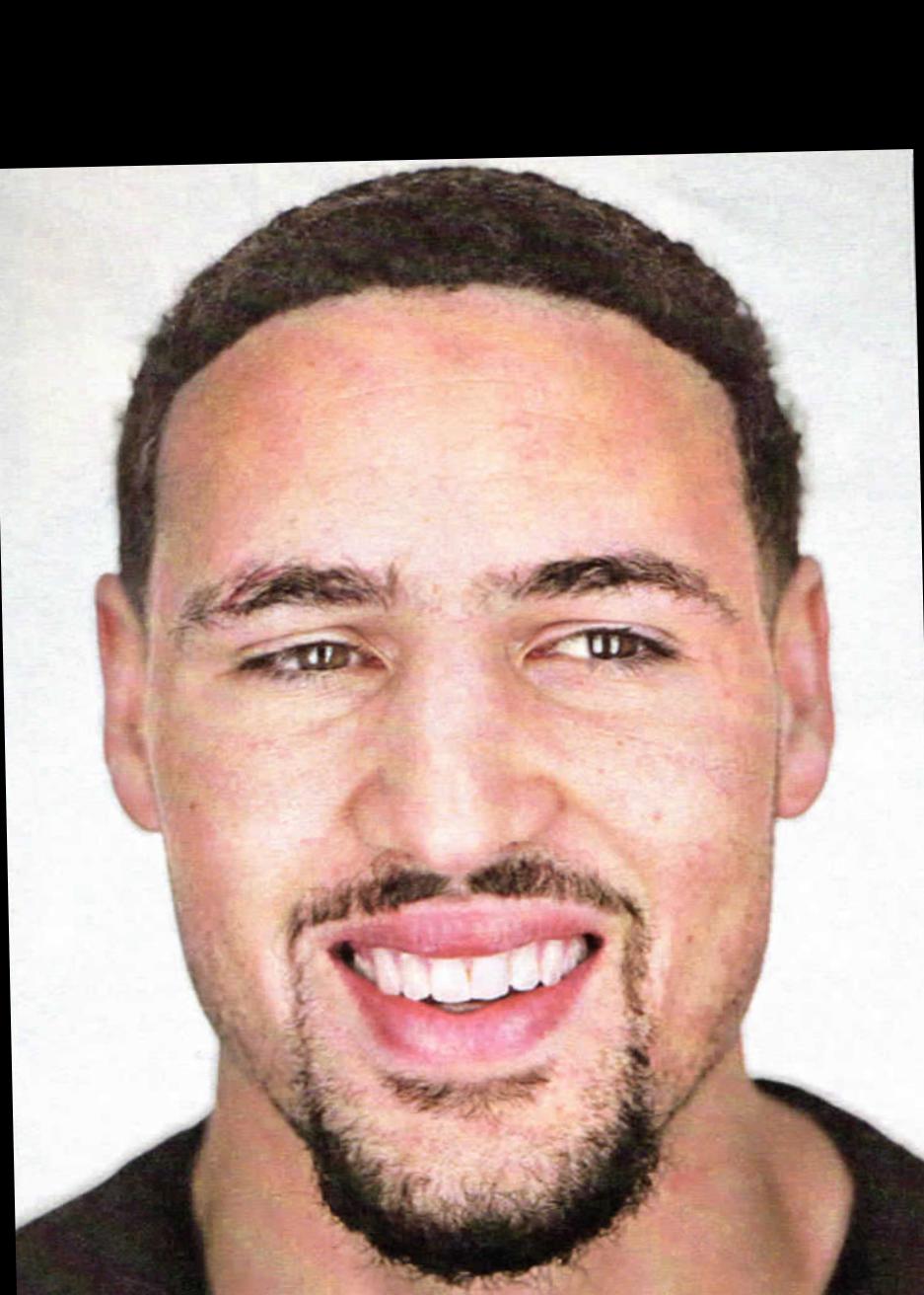
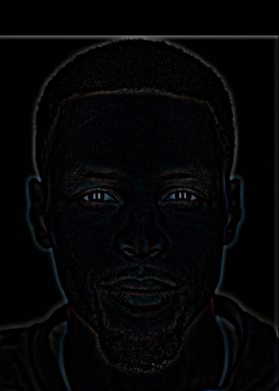
This one of the Splash Brothers (Stephen Curry and Klay Thompson) is my favorite:

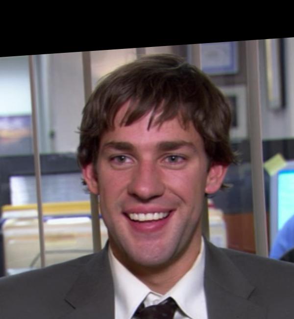
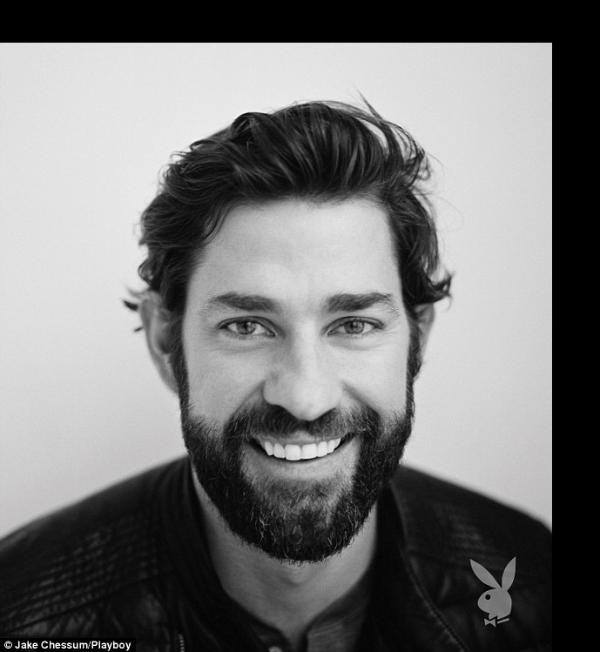
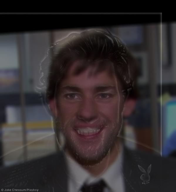
Below is a hybrid of Jim and John, which I thought could have looked better since the angles of the two portraits are different, so the features do not line up too well.

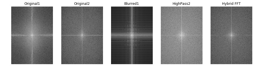
Fourier (Frequency) analysis

Here we illustrate the process of creating the 'Splash Brothers' piece by showing the log magnitude of the Fourier transform of the two input images, the low-pass filtered image, the high-pass unsharp filtered image, and the hybrid image, from left to right.

Part 1.3: Gaussian and Laplacian Stacks

An image pyramid is a multi-scale representation of an image, with each level a result of the image being resized to different factors (filtering and downsampling). A stack is similar to a pyramid; however, the images are never downsampled so the results are all the same dimension as the original image, and can all be saved in one 3D matrix (if the original image was a grayscale image).

In a Gaussian stack, subsequent images are blurred by convolving the image with a Gaussian kernel. A Laplacian stack is constructed from the differences between levels of the Gaussian stack. The last level of the Laplacian stack is the last level of the Gaussian.

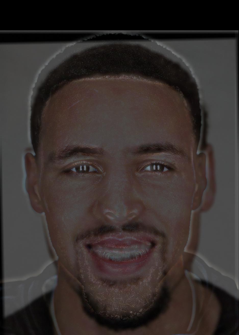
By visualizing the Gaussian and Laplacian stacks for images that contain structure in multiple resolutions (such as our hybrid images above), we can observe the structure at each level. Below are the Gaussian stacks (top) and Laplacian stacks (bottom).

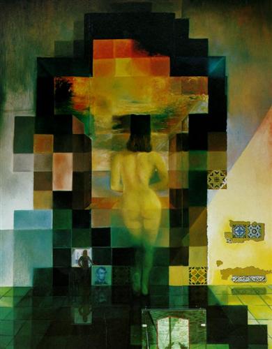
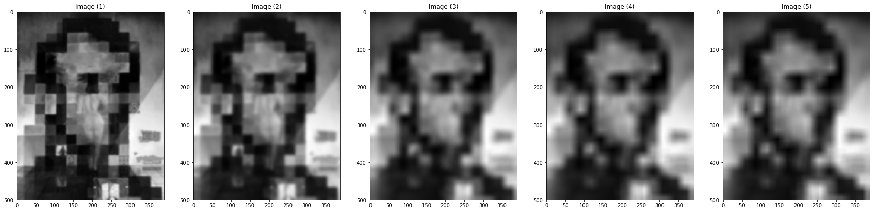
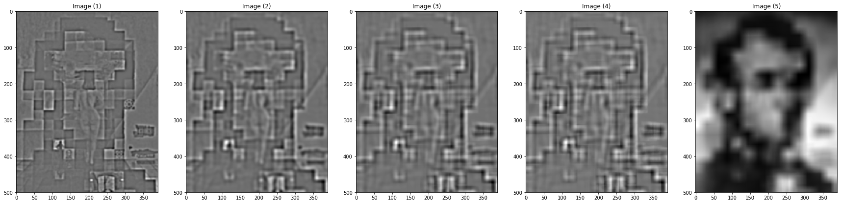
At the deeper levels of the Laplacian stack, Lincoln can be seen more easily; at the shallower levels, the artist's wife can be more easily seen.

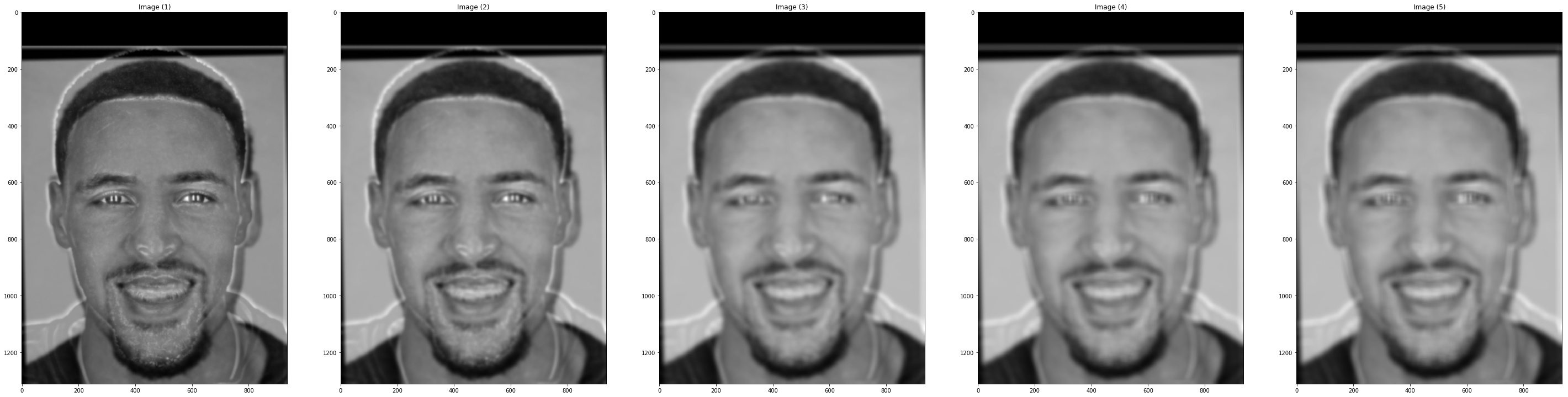
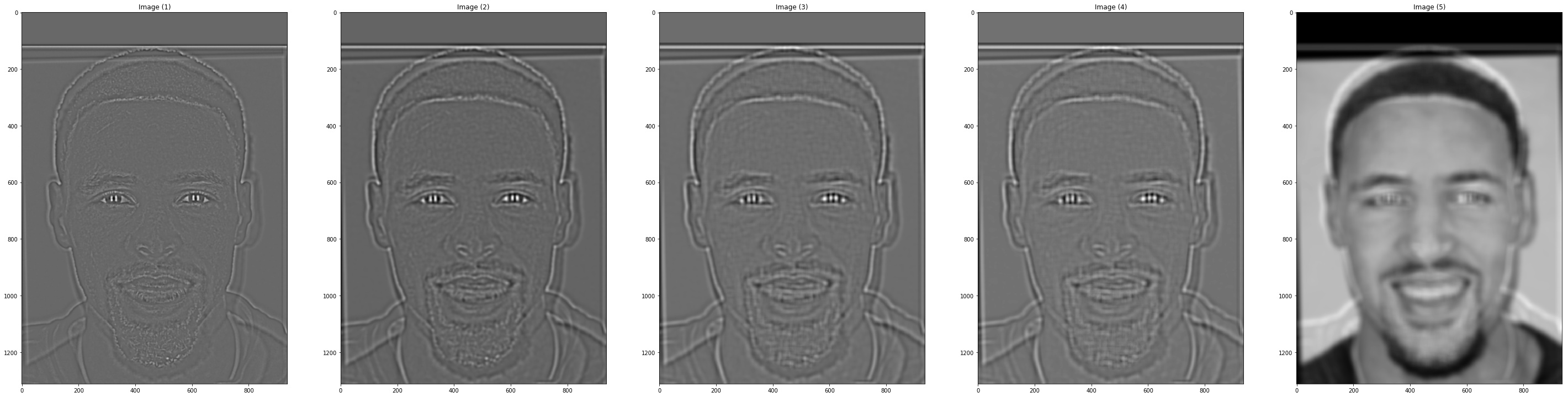
The first Splash Brother (high-frequency Steph) is visible at first, then the second Splash Brother (low-frequency Klay) becomes visible.

Part 1.4: Multiresolution Blending

The goal of this part of the project is to blend two images seamlessly using a multi resolution blending as described in the 1983 paper by Burt and Adelson. An image spline is a smooth seam joining two image together by gently distorting them. Multiresolution blending computes a gentle seam between the two images seperately at each band of image frequencies, resulting in a much smoother seam.

For input images A and B (of the same size), build Laplacian stacks $ LA $ and $ LB $.
Create a binary-valued mask M representing the desired blending region.
Build a Gaussian stack $ GM $ for M.
Form a combined stack $ LS $ from $ LA $ and $ LB $ using values of $ GM $ as weights. That is, for each level $ \ell $, $LS_{\ell}[i,j] = GM_{\ell}[i,j] LA_{\ell}[i,j] + (1 - GM_{\ell}[i,j]) LB_{\ell}[i,j].$
Average the levels of $ LS $.

Blended images in color (Bells and Whistles) are shown below:

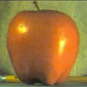
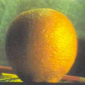
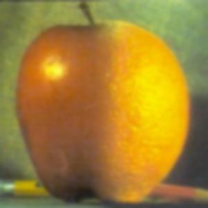
The Laplacian stack of the orapple is shown below.

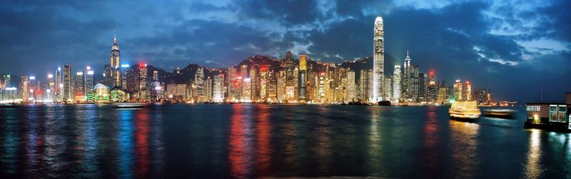
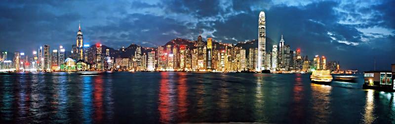
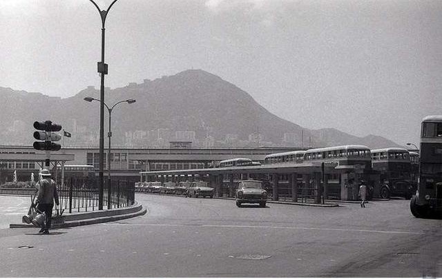
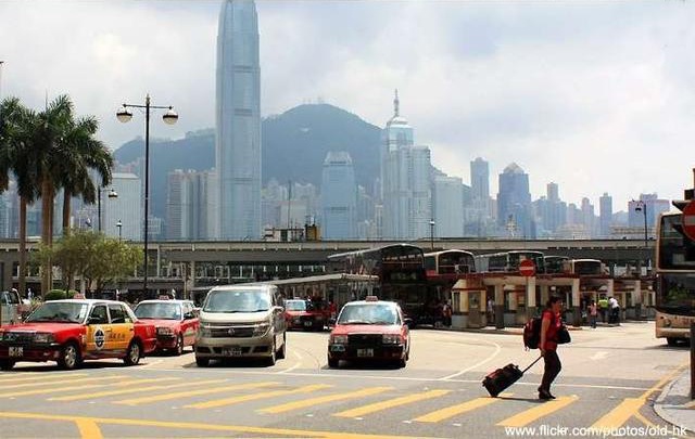
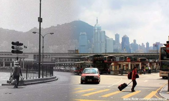
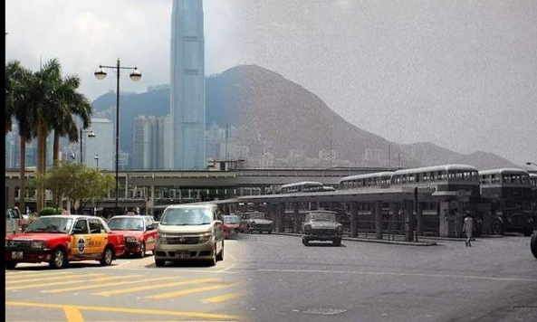
Some really nice shots of old blended with Hong Kong below.

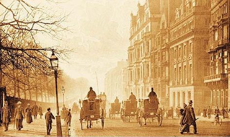
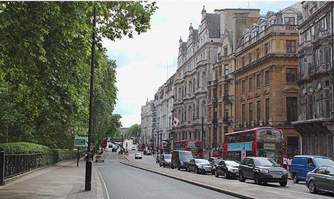
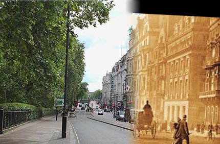
And now for old versus new London.

Part 2: Gradient Domain Fusion

Part 1 focused on frequency domain processing to generate hybrid and blended images, as well as to explore different structures with Laplacian stacks. In Part 2 below, I explore gradient-domain processing, specifically utilizing Poisson blending to seamlessly blend an object from a source image to a target image. To avoid obvious seams, we focus on preserving the x and y gradients of the source image. Since humans generally care more about the gradients than the actual intensity values, we use least squares to find values for the target pixels that most closely match the gradients of our source image. In addition, the newly computed pixels should have a similar color profile to the target image due to the boundary conditions.

However, since we do not optimize for preserving the specific intensity pixel values of our source image, the color of the pasted image could be different from the color of the original image.

Part 2.1: Toy Problem

Let's get started with a toy problem. To get started with gradients, we will reproduce a small grayscale image of Woody and Buzz by matching the x and y gradients from this toy image, and finally matching the intensity of the top left pixel to the original toy image to obtain a unique solution to our least squares optimization. The original image is on the left, and the reconstructed image is on the right.

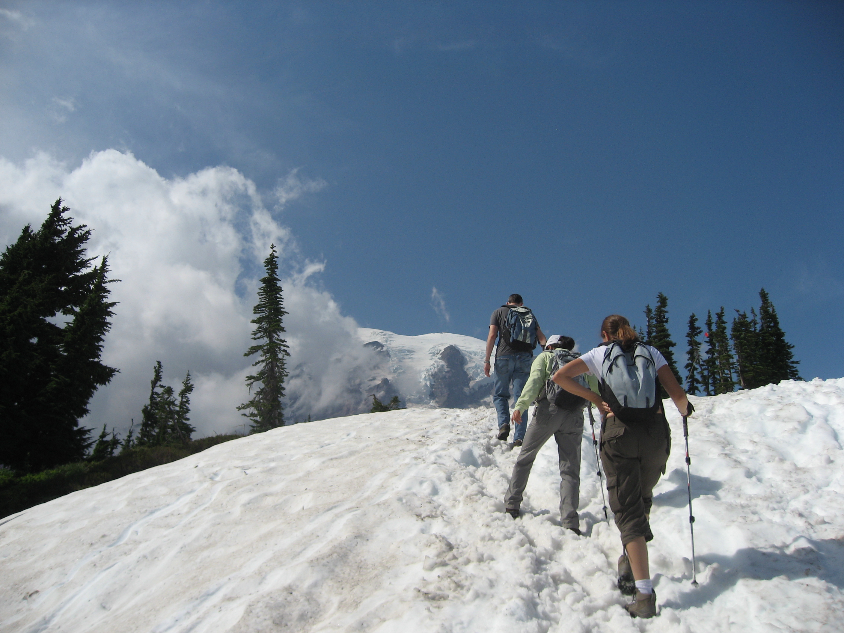
Part 2.2: Poisson Blending

Background

Now for the fun part: smooth, seamless Poisson blending of a source image into a target image. First, two masks are needed: one for the region of the source image that we want to paste into our target image, and one for the desired destination location of this pasted source region. Next, we solve for the pixels specified by the source mask by minimizing the least squares difference of the gradient of the pixels in the target region and the source region, as well as minimizing the least squares difference between the gradient at the boundary of the region and the source region boundary. These pixels are then copied into the target region specified by the target mask for a seamless blend.

Formally, given the pixel intensities of the source image $ s $ and of the target image $ t $, we want to solve for new intensity values $ v $ within the source region $ S $ (as specified by a mask):

$\mathbf{v} = \text{argmin}_{\mathbf{v}} \sum_{i \in S, j \in N_i \cap S} \left( (v_i - v_j)^2 - (s_i - s_j)^2 \right) + \sum_{i \in S, j \in N_i \cap \neg S} \left( (v_i - t_j)^2 - (s_i - s_j)^2 \right)$

In the above minimization problem, each $ i $ is a pixel in the source region $ S $ and each $ j $ is a 4-neighbor of $ i $ (left, right, up, and down).

Results

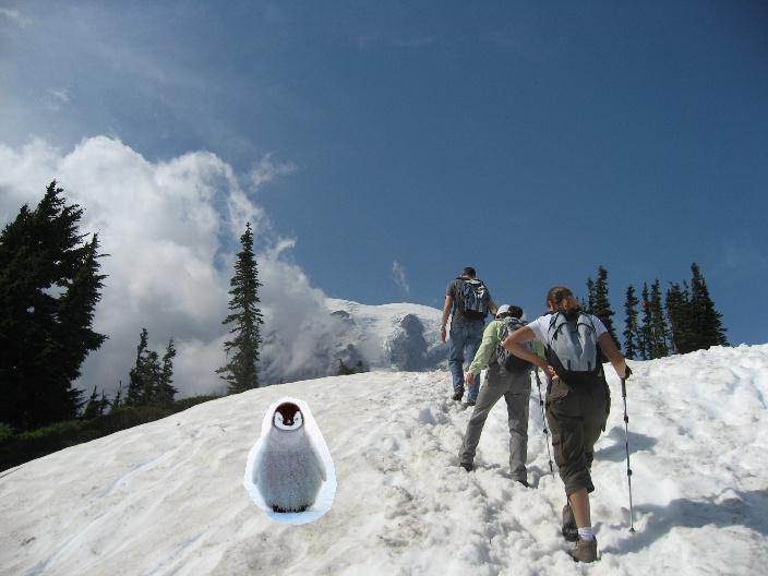
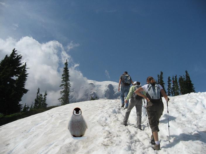
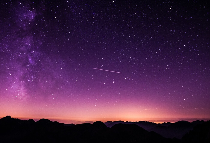
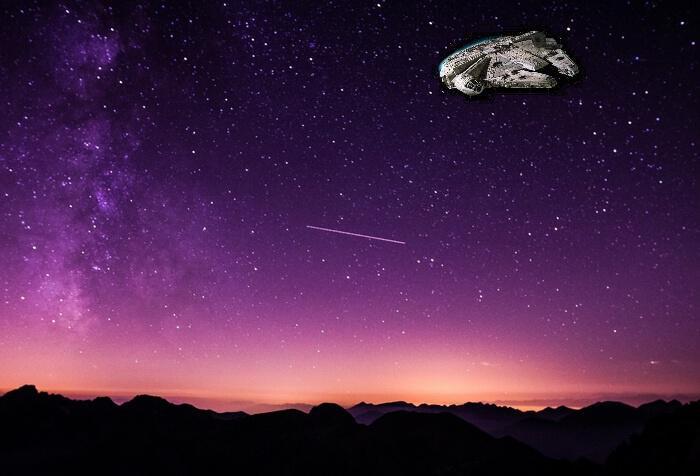
Below are several blending examples, with:

the source mask and source image; target image; the naive blended image with the source pixels directly copied into the target region; and the final Poisson blend result.

This one of dolphins next to a sailboat didn't work out too well:

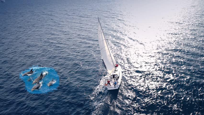
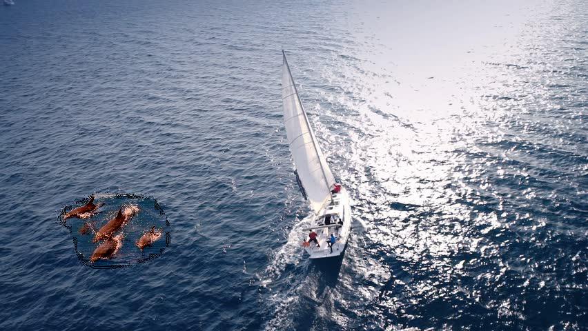
There is a decent color difference between the sea around the dolphins and the water that it was pasted into, which results in a color change for the dolphins. The texture of the water around the dolphins is also different from that around the sailboat. The gradients are preserved, but the color is changed. With the right source image that matches the sailboat water better, the result would have been better.

Below are Poisson blended images vs. multiresolution blended images.

Takeaways

I love the results from this project. I have always wanted to create blended images of old and new Hong Kong, which is where my family is from. However, this project was absolutely incredibly time consuming, and I learned that there is no fixed recipe for obtaining good blending results. There are many different methods for blending, and various parameters for different pairs of images. It would have been nice to have more time to experiment around to try and get the best results. Definitely polished my python, scikit-image, and numpy skills!