We proceed by first creating a gaussian filter, convolving it with an original image to get a low-pass. Then subtract the result of the convolution from the original image to see the visible high-frequencies. Then we take our original image and add back a cutoff scaled version of the high frequencies to sharpen our image. See images below for results:
Original Image
Result of convolution with Gaussian Filter
High Frequencies
Sharpened Final Image
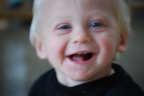
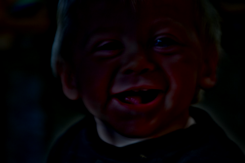
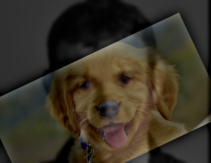
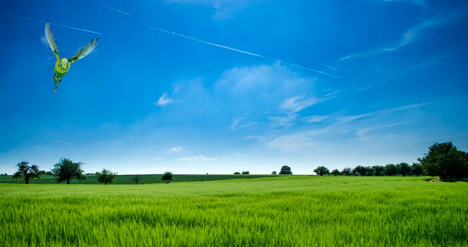
We proceed by low-passing our original image, then high-pass filtering our second image. We use Gaussians with specific cutoff frequencies that we hand-pick to achieve the best result. Finally, we take an average of the low-pass and high-pass to achieve our final hybrid. I have also attached frequency plots below. See images below for results:
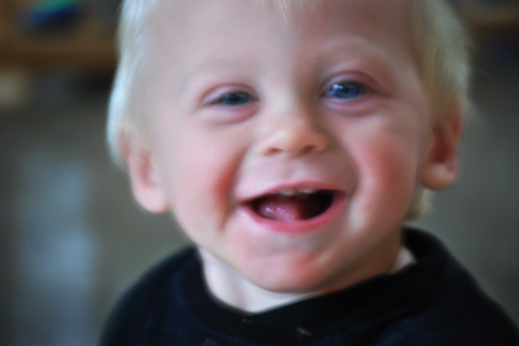
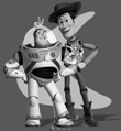
Image 1

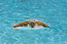
Image 2
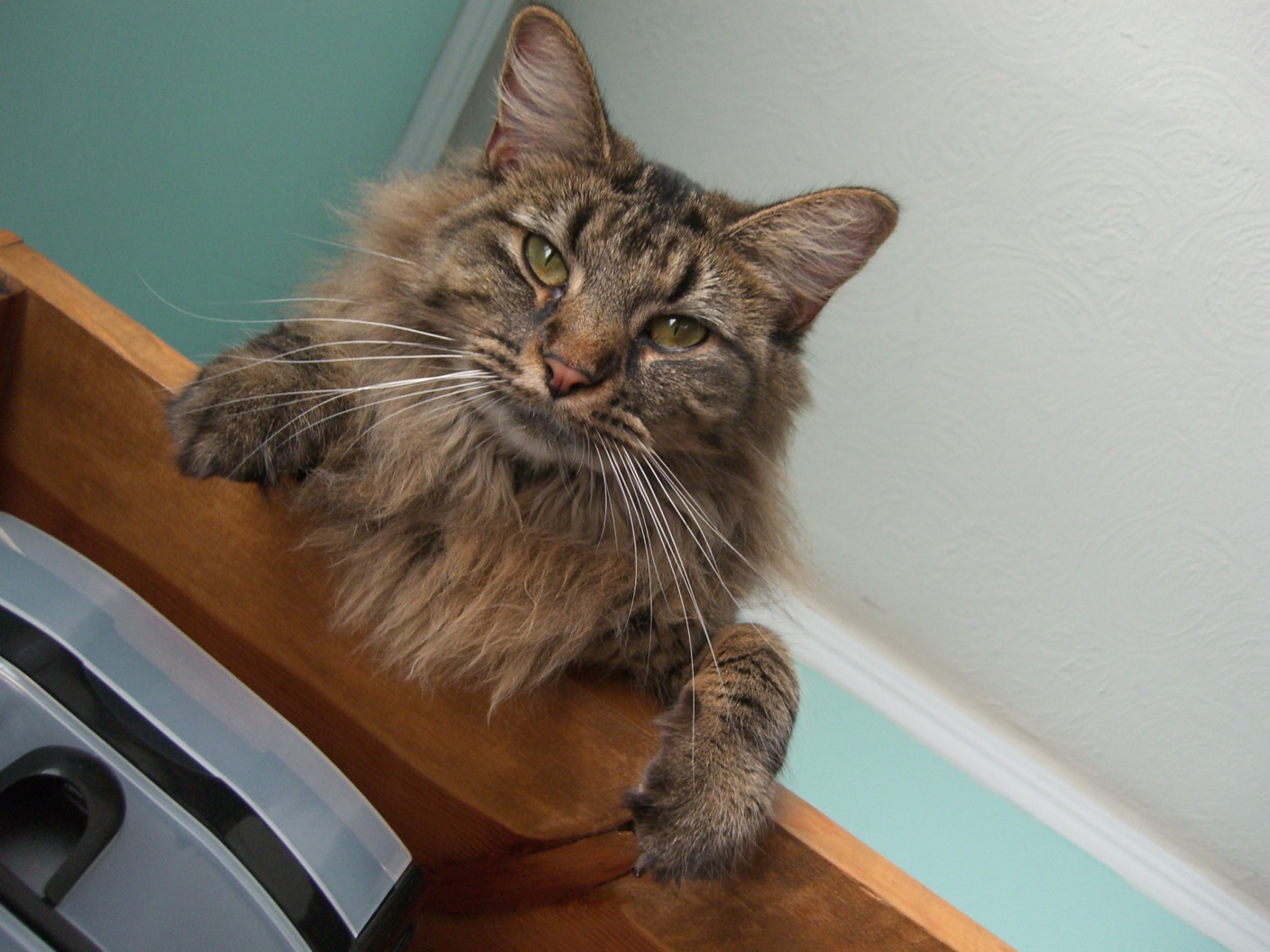
Hybrid Image
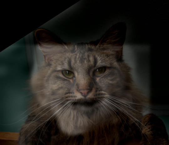
Image 1
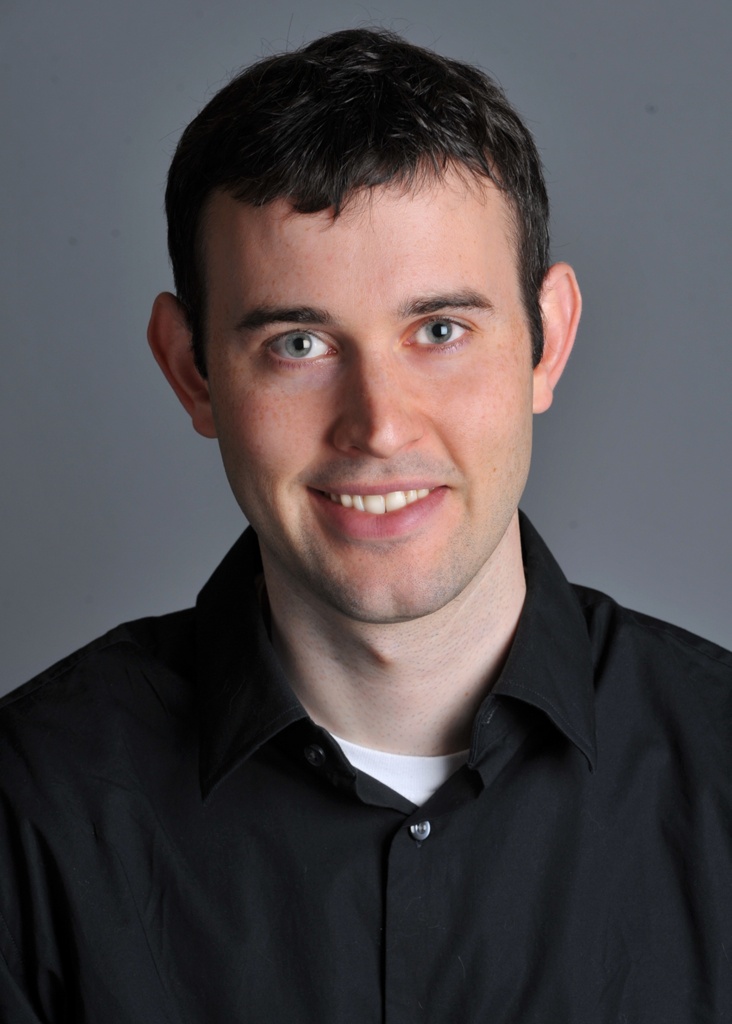
Image 2
Hybrid Image
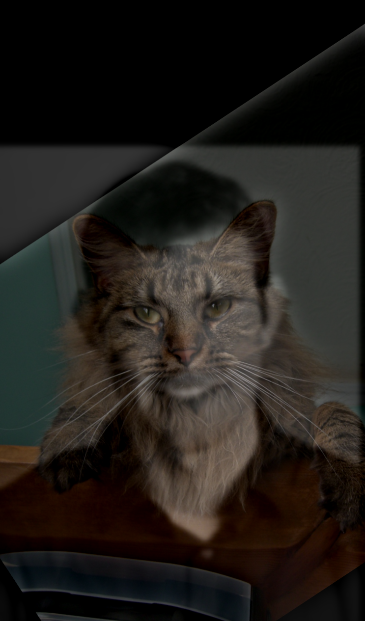
Image 1
Image 2

Hybrid Image
Input Image 1 Frequency
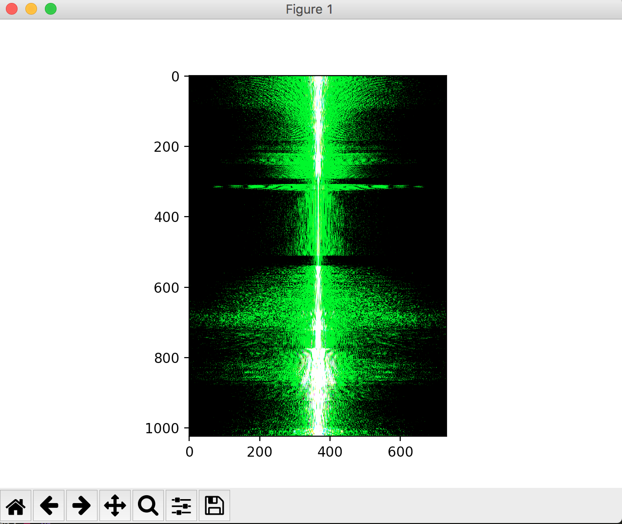
Intput Image 2 Frequency
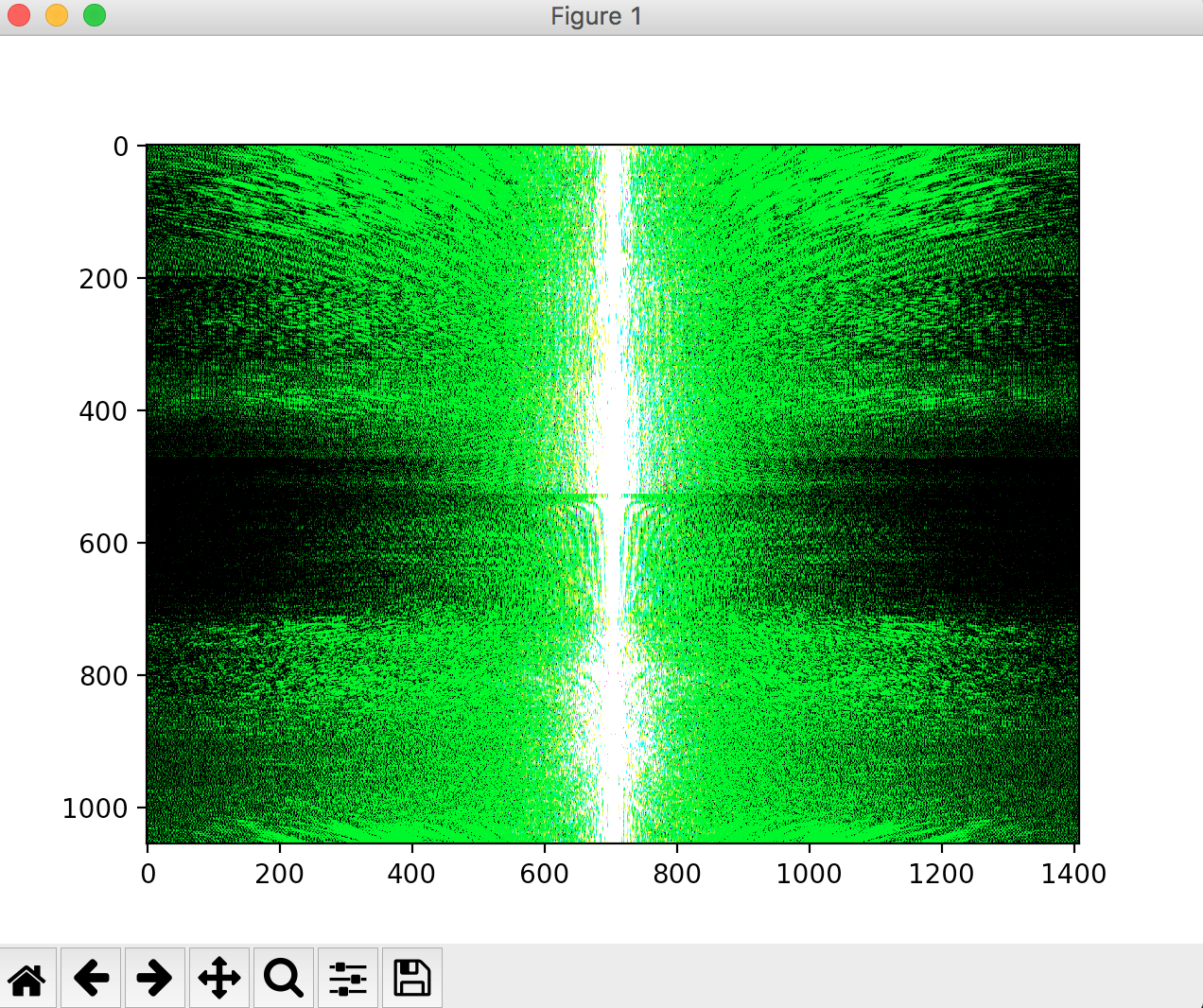
Low-Pass Frequency
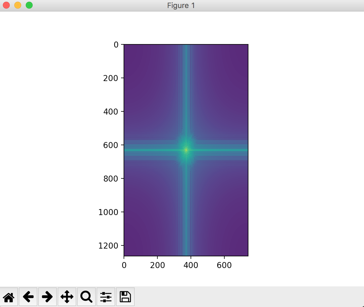
High-Pass Frequency
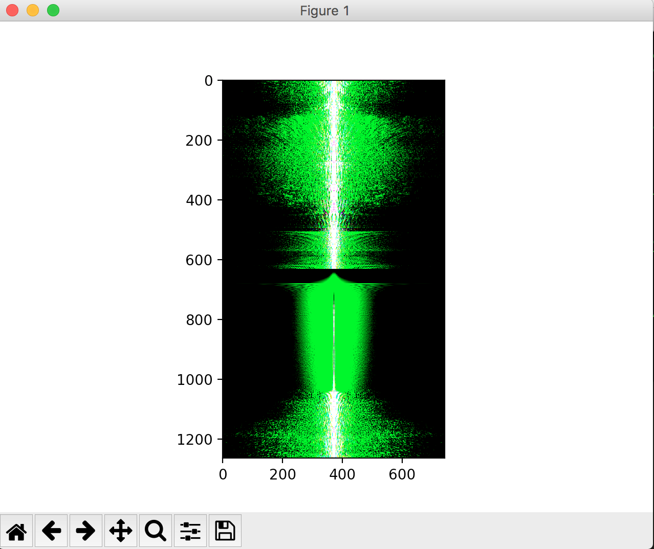
Hybrid Image Frequency

This part of the project focuses on gradient-domain processing, which allows us to seamlessly blend an object or texture from a source image into a target image. While copying and pasting pixels from one image into another is feasible, this ends up creating seams on the edges, which is not ideal. Instead we can formulate this "copying and pasting" into a least squares problem that we can then solve. The equation for this least-squares problem is listed on the course website.
We can simplify the equation shown in the general case, to have one source image and simply attempt to reconstruct that image using a least-squares problem. See images below for results:
Original Image
Reconstructed Image

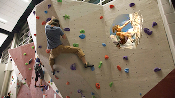
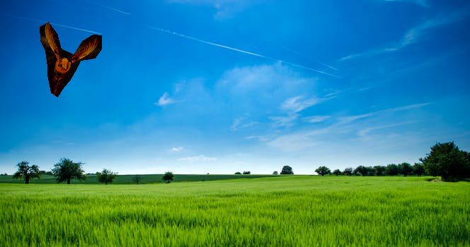
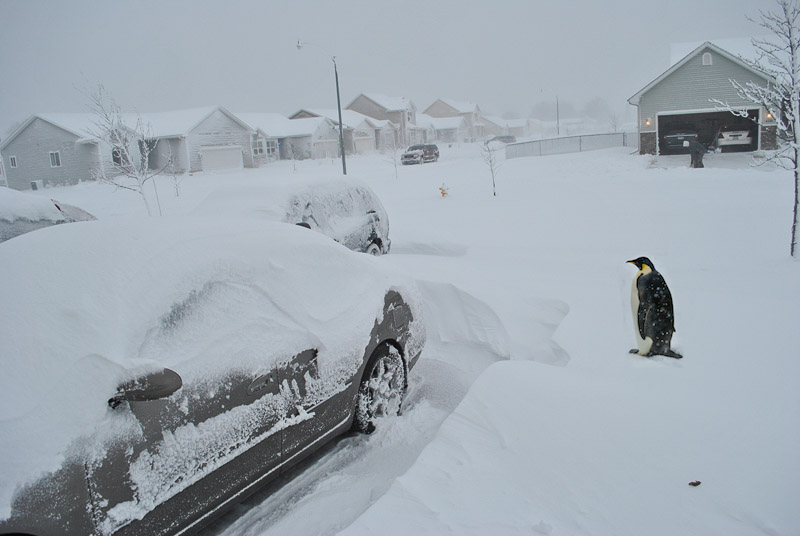
Below, I have included 4 results from the poisson blending that I used. I did all these blendings my solving the least squares problem indicated on the 194 course website. First I generated a mask of the source image generated by a polygon shape I drew (Credit: Nikhil's Python Starter Code). Once I had the mask of the source image, I aligned it with the target image and applied it to get a target image mask (Pixel values of 1's where the source image would be placed and 0's elsewhere). I used these masks as well as the original source and target images and created matrix A and vector b to solve the more complicated optimization problem as a simple Ax = b least-squares. From there, I used a scipy sparse matrix solver to generate the x vector, which I then plugged into the target image mask. During the process of generating x, I calculated the gradients within the mask and the edge gradients comparing the source image polygon to the target image edges, thus being able to smoothe the edges between the source image polygon and the target image. As a result, I was able to generate the following 4 results.
The first three results work very well, as the source image cutout seems to be blended nicely into the target image (at least visually appealing to the human eye). However the last blended result ends up being a failure case because the background of the target image (essentially a beige colored wall) does not mesh with the source image background (a climber in the foreground with blue sky in the background). The color difference results in a terrible resultant gradient between the edge of the source image and the edge of the target image mask, which results in an inability to blend the two effectively. We can see this via the human eye in the image because we can clearly distinguish that the climber is not part of the original wall image.
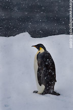
Source Image

Target Image

High Frequency Cutout Directly onto Target Image
Output Fully Blended
Source Image

Target Image

Output Fully Blended
Source Image
Target Image

Output Fully Blended
Source Image

Target Image

Output Fully Blended