Project 3: Frequencies and Gradients

Part 1: Frequencies

Part 1.1 Sharpening

By subtracting away the low frequencies, we are left with high frequencies (edges). We can add these edges back to the original image with a weighted constant to accentuate all the edges of the image and make the higher frequencies more intense.

Part 1.2 Hybrid Images

We achieve hybrid images by overlaying a high frequency image with a low frequency image. These two images are created using a high pass filter and a low pass filter, respectively. From a far distance, we can see only the low frequency image, and up close, we can see only the high frequency image.

Part 1.3 Gaussian and Laplacian Stacks

The Gaussian stack was simply a stack of images, where each image i was the Gaussian filtered image (i-1). The LaPlacian stack was a stack of images where image i was the G[i] - G[i+1], getting the differences between the higher frequency gaussian image and the lower frequency gaussian image.

Part 1.4 Multiresolution Blending

Using the algorithm from the paper, multiresolution blending works by taking the two LaPlacian stacks of the original image and blending them together while using a Gaussian mask. The mask lets us blur together the seams of the two images so that the transition becomes smooth.

Part 2: Gradients

This part of the project is essentially trying to make sure that gradient stays the same from image to image. Naively copying the image over makes the gradient change very suddenly, and this is what causes it to look bad. However, if we formulate the problem as a least squares, we can spread the error out over the entire image so that the change in the gradient is the least noticeable. This way, changes from the target region to the source region are minimized and the image looks very complete.

Part 2.1 Toy Problem

Used gradients to reconstruct the toy image

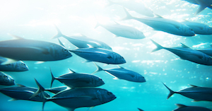
Part 2.2 Poisson Fusing

The blue background of the fish picture and the blue background of the ocean don’t match exactly. However, by doing least squares, the colors of the fish picture are changed so that they match the color gradients of the ocean.

The jelly fish did not blend well. Although there is no visible edge, the colors are skewed to account for the changing gradient. The original jelly fish used to be orange and now it is a neon green.

The jelly fish did not blend well. Although there is no visible edge, the colors are skewed to account for the changing gradient. The original jelly fish used to be orange and now it is a neon green.

The two have very different results. The laplacian blending is more suited for combining entire parts of the image together, and we can see that the color gradient is not preserved and there is a visible spot where the two images change. With poisson, we have more flexibility and can actually blend the image with color accuracy by making the gradient change smoother.