
In part 1, I explored using frequencies to blend together and merge images.
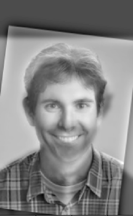
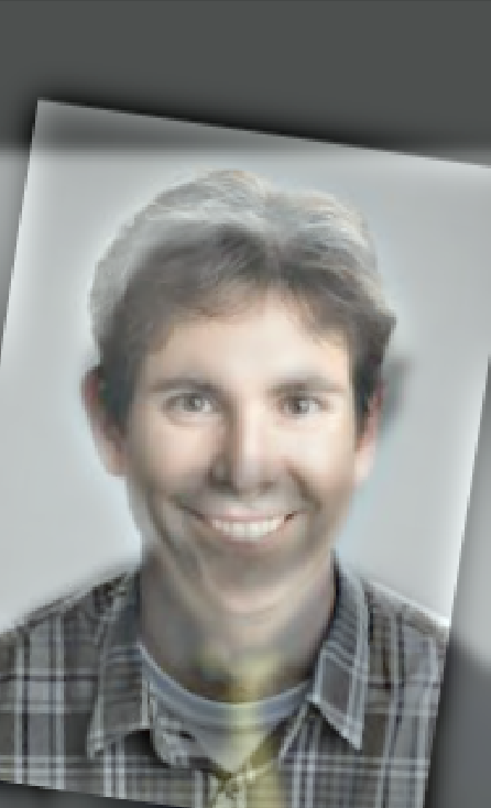
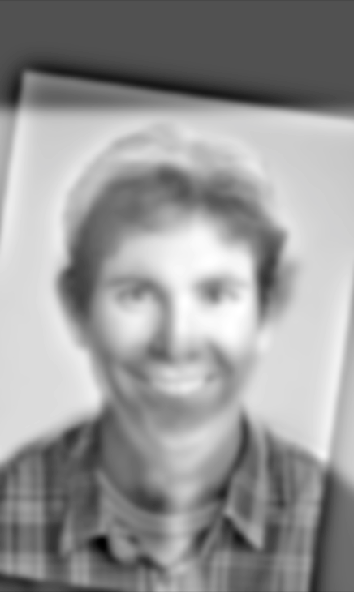
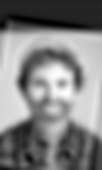
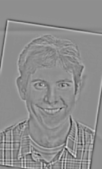
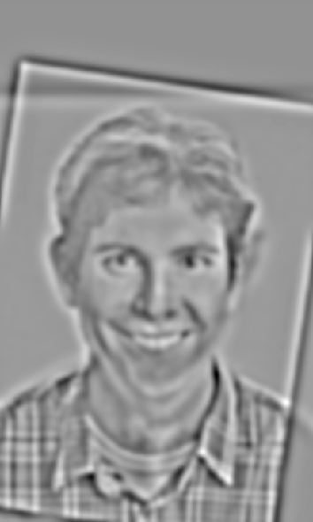
For the warmup, I used the unsharp mask technique. The general idea is to first extract the details of the image by subtracting the blurred image from the original image. The next step is to add a scaled factor of these details back to the original image. To get the blurred image, I used a Gaussian filter of kernel size 25 and sigma 5. Then, I multipled the details by an alpha of 0.5, and I added this to the original image to get the final result.
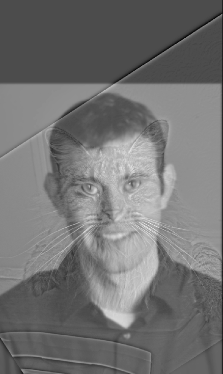
To create a hybrid image, I had to extract the high frequencies of one image and the low frequencies of another image. After combining these frequencies into one image, the idea is that you can prominently see two different images depending on the distance at which you are viewing the combined image. When you view the image at a close distance, the high frequency image dominates your perception. When you view the image at a far distance, the low frequency image dominates your perception. For example, in the first row of the following pictures, we use a low pass filter on the Derek image and a high pass filter on the Nutmeg image to get the combined result.
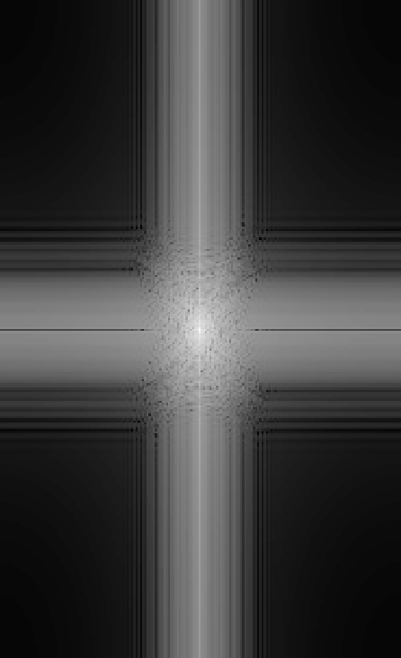
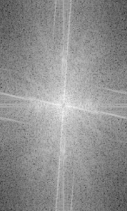
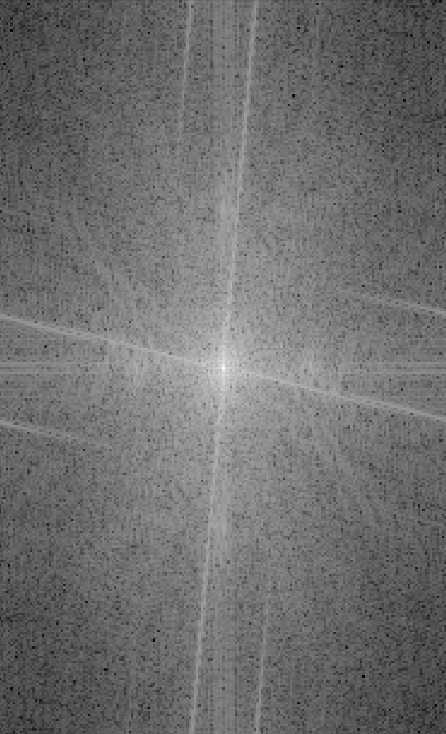
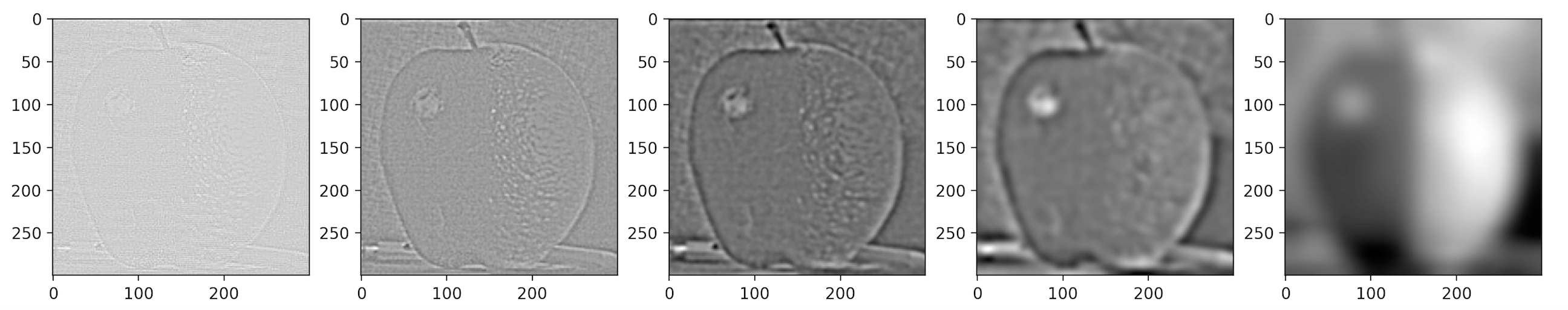
The following are the fourier transforms for the grayscale hug image, grayscale denero image, low pass filter on the hug image, high pass filter on the denero image, and the hybrid image.
The combined image of Oski and Dirks failed to match well mostly due to the angle positioning and shape of the two heads. Dirks' head is angled compared to Oski's head, making Dirks' head not have features laid out in a format that is as similar to Oski's head features. Thus, part of Dirks' head juts out past Oski's face in the hybrid photo, and the features like the smile don't align that well.
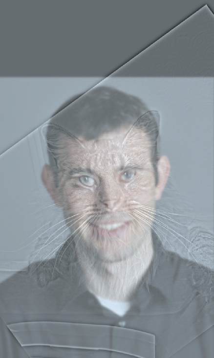
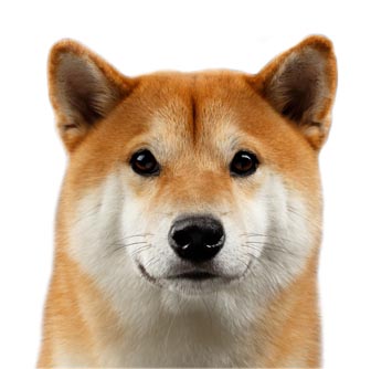
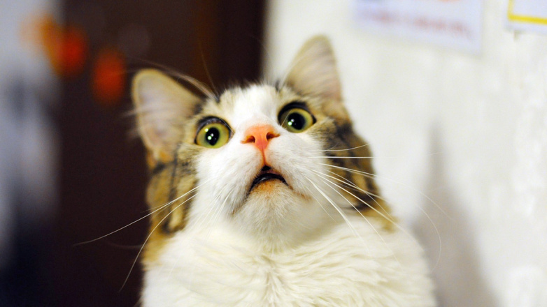
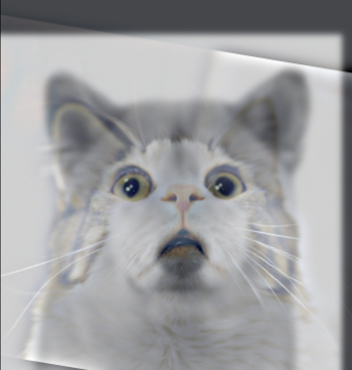
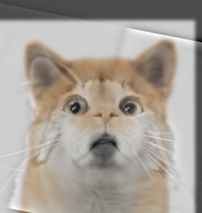
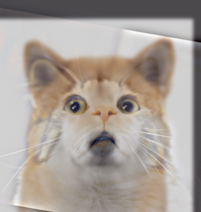
When using color to enhance the effect, it seems to work better to use color for at least the low frequency component. Additionally including color for the high frequency component is not as crucial. You can see this in the following shiba and cat images. Since the low frequency image forms the background, it looks better to at least have the low frequency image be colored. There doesn't seem to be as significant of a difference when both frequencies are colored versus just having the low frequency be colored (Compare the middle and right images in the second row).
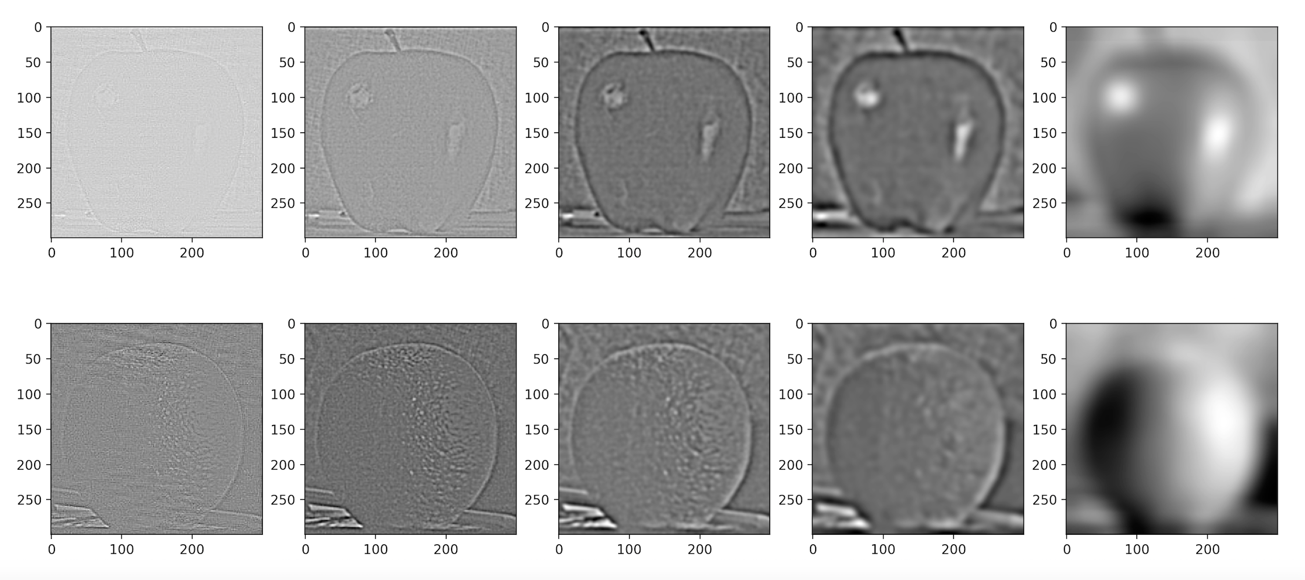
In this part, I created Gaussian and Laplacian stacks. The Gaussian stacks act as low pass filters and reveal the low frequencies in the image. The Laplacian stacks act as high pass filters and reveal the high frequencies in the image. I used a stack level of 5. When using the Gaussian filter, I used kernel size 41 and sigma's that increased by a power of 2. Thus, the first Gaussian stack used a Gaussian filter with a sigma of 1, the second one used a sigma of 2, the third one used a sigma of 4, etc. The Laplacian stacks are created by taking the difference between two layers of the Gaussian stack. It's important to note that the last stack in the Laplacian stack is the same as the last stack in the Gaussian stack. This is so you can sum the layers of the Laplacian stack to get back the original image.


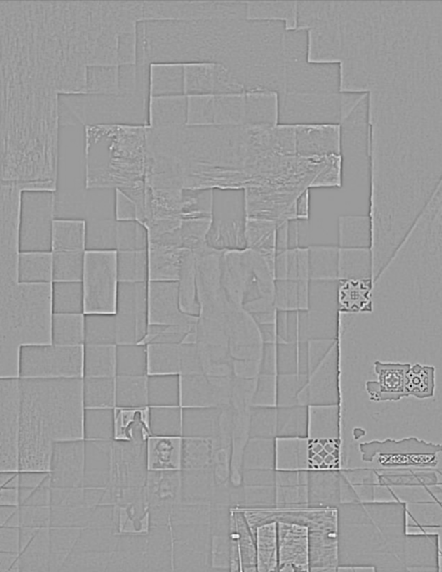
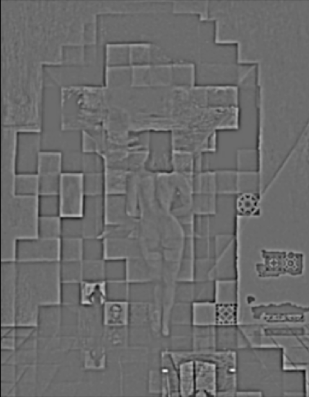
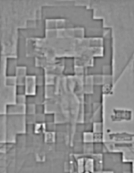
Let's take a look at the gaussian and laplacian stacks on the Hug Denero hybrid image. The Gaussian stack shows Hug more prominently, which is expected because it emphasizes low frequencies. The laplacian stack shows Denero more prominently, which is also expected because it emphasizes high frequencies.

I used the laplacian and gaussian stacks to implement multiresolution blending. I first created laplacian stacks for the two images I wanted to combine. Then, I created a mask for the region in the images I wanted to blend together and also created a gaussian stack for this mask region. Finally, I formed a combined stack by utilizing both laplacian stacks and nodes of the gaussian stack as weights. By summing the layers of the combined stack, I was able to get the final result of the blended images. I used the same stack parameters as part 1.3 to generate my gaussian and laplacian stacks.


The goal of part 2 is to move part of a source image onto a target image, minimizing the seam between the source image portion and target image. It is bad to just directly copy the pixels because there will be a clear border between the source image portion and the target image. One strategy to accomplish this goal is Poisson blending. To do this, I set up a linear least squares equation that solves for the new source image values once it's placed in the target image. These new source image values will maximally preserve the gradient of the source region without changing the background pixels. By trying to preserve the x and y gradients, the seam between the source image portion and target image portion becomes a lot less noticeable. It's important to note that people typically care a lot more about the gradient of an image rather than the overall intensity, and the Poisson blending technique is based on this observation.
Given a source image, I am using gradients plus one pixel to reconstruct a new image that should recover the source image. I am trying to solve for each pixel of the new image by using the following constraints: the x-gradients and y-gradients should closely match the x-gradients and y-gradients of the source image, and the top left corner pixels of the source and new image should also closely match.
The goal was to try to seamless blend a portion of a source image into a target image. I solved for the new source image pixel values using constraints similar to the ones in Part 2.1. However, instead of trying to minimize the difference between the top left pixels as in Part 2.1, the constraint tried to minimize the difference between the edge pixels of the source image and the pixels at the edges of the target image where the source image would be placed.
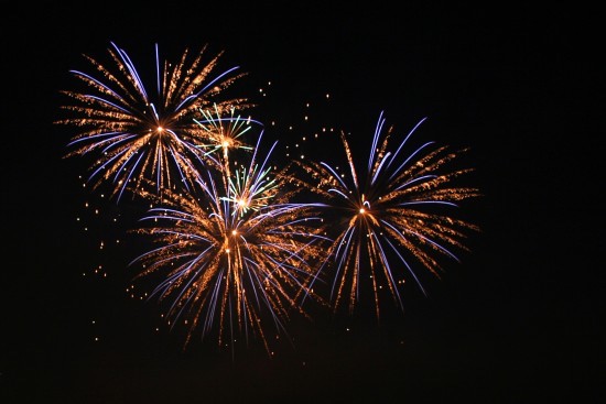
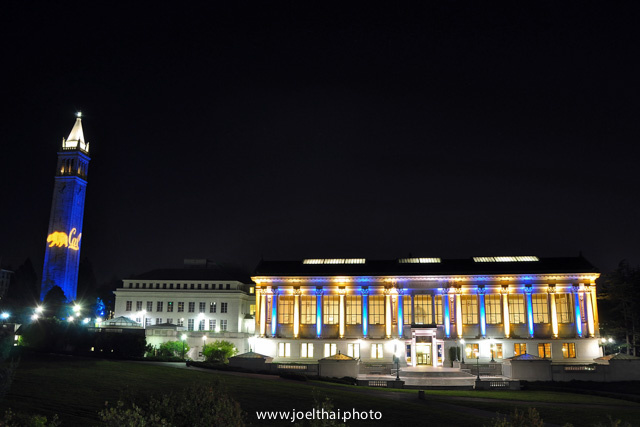
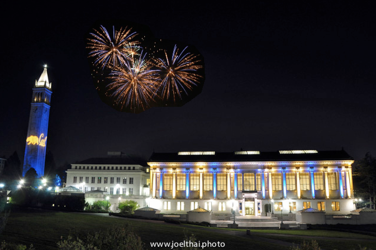
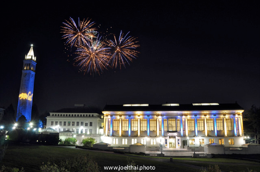
To get the campanile and fireworks combination, I had to first create a mask for the portion of the source image I wanted to transfer (just the area around the fireworks). I also created a mask for where the source image would be placed in the target image. Then, utilizing information about pixel placement in both of these masks, I used the technique in the previous paragraph to solve for the values that the firework would be in the target image. I then copied the solved values into the target image, knowing where I should place these solved pixels based on the target image mask.
You can notice below that when the fireworks pixels are directly copied, you can see a distinct black border. However, with the poisson blending technique, the fireworks blend into the gradient of the background sky.
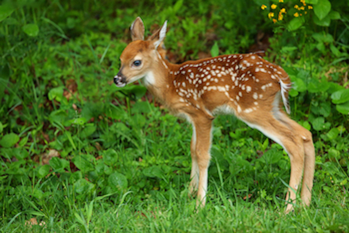
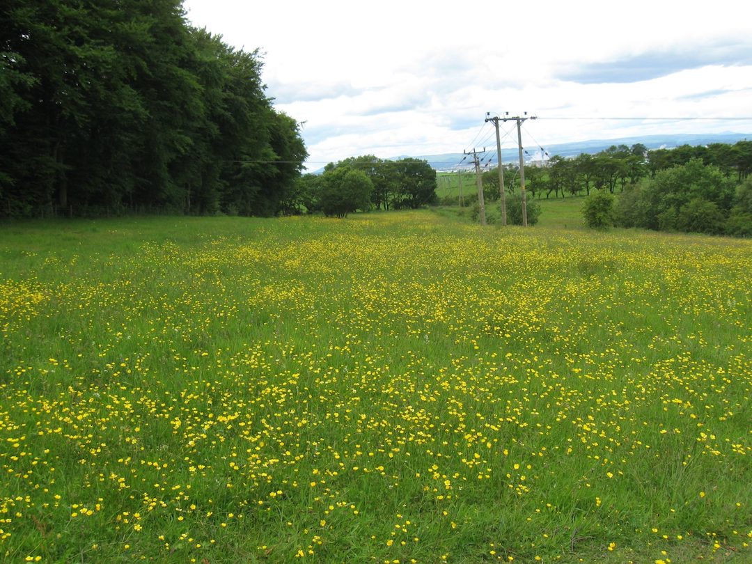
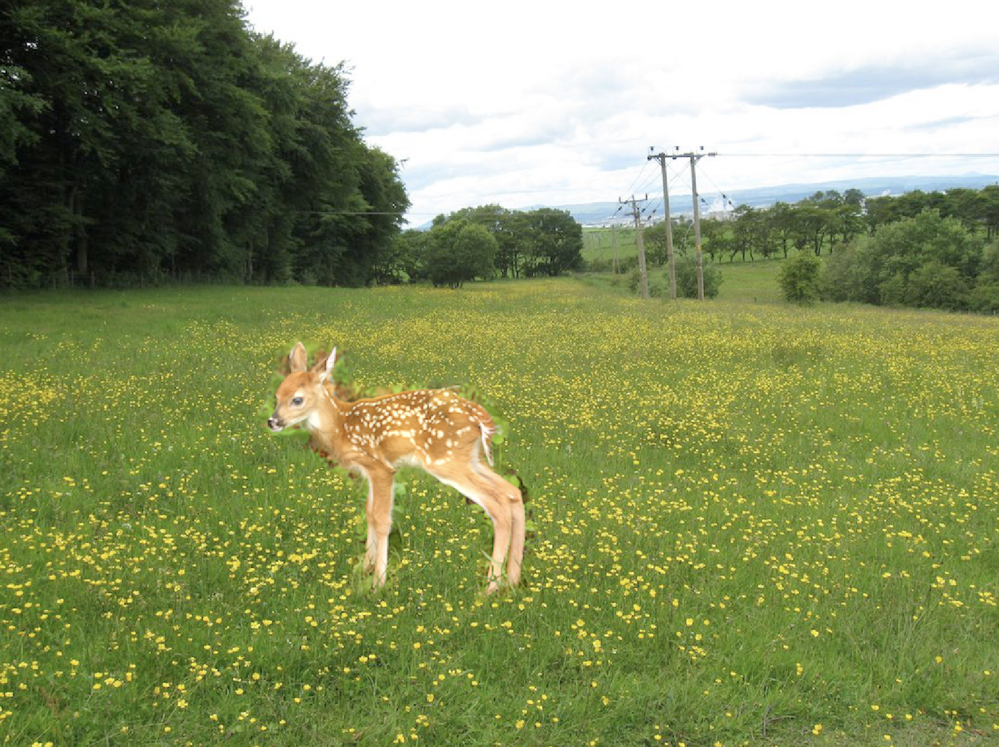
You can pretty clearly see the outline of the deer image against the meadow background, especially around the top and back of the deer. This likely failed because although the colors were similar, both the source and target image had very textured backgrounds. Due to these textures, it was hard for the source image to change its grass texture around the deer to map to the grass texture of the meadow.
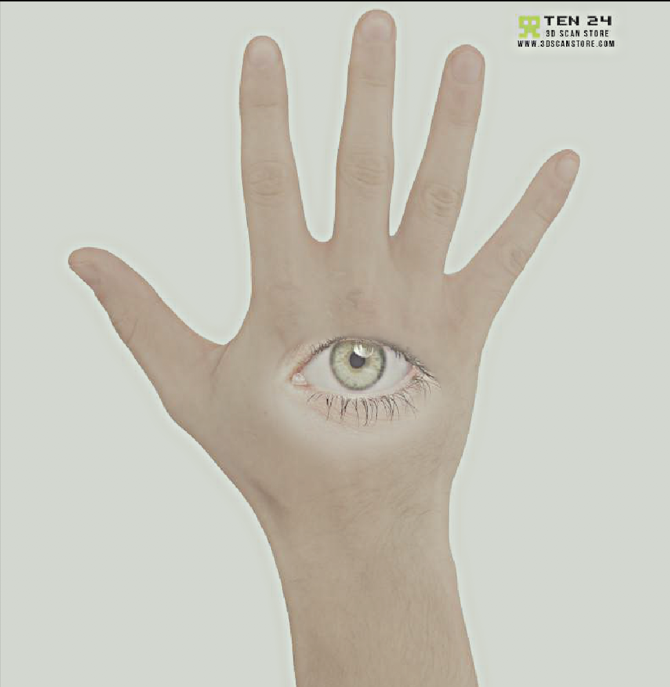
You can see that laplacian blending provides a smoother transition between the seams. For example, the top eyelid crease in the laplacian blending technique is almost virtually gone. This is because the laplacian blending process utilizes a gaussian filter, which will blur the boundaries at the seams and provide this smoother transition. Also, poisson blending minimizes the change in gradient between the source and target images, which means it might not preserve the original intensity of the source image. Thus, it is more appropriate to use the laplacian stack blending technique if you want to preserve the colors of the source image.
One of the most important things I learned from this project was the importance of how you could speed up your code and process images faster. For example, by using vectorization and sparse matrices, I was able to speed up computation and save memory when dealing with images. It was a new way of programming for me to try to minimize the use of for loops. There were also simple wins to speed up the process, such as resizing the images to be smaller than their original downloaded size.