CS194-26:
Image Manipulation and Computational Photography
Grace Park
SID: 3032341209
cs194-26-acd
Project 3: Fun with Frequencies and Gradients!
Purpose
The purpose of this project was to understand the effects of manipulating frequencies of the images. Blurring, sharpening, blending of two images can be done from the process.
Part 1: Frequency Domain
Part 1.1: Warmup
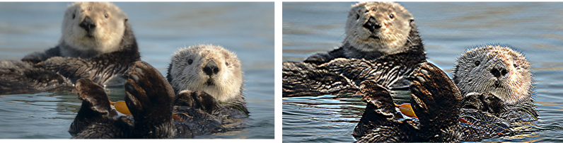
Sharpening image using Gaussian Filter and Laplacian Filter.
The idea here is that we use a gaussian filter to produce a high frequency image of the original image and add it to the original so that the high frequencies are emphasized. This results in a sharpened image.
The kernel size and the sigma for the Gaussian Filter is chosen according to the image.
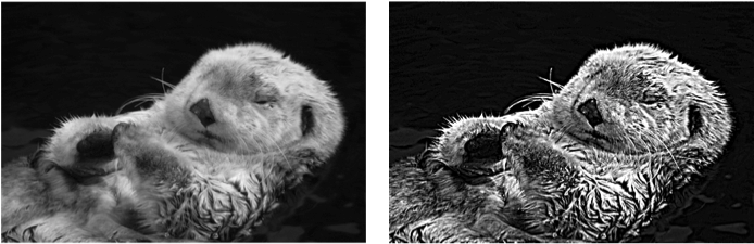
Example 2: Sea Otter Color
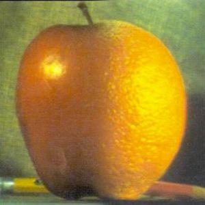
Part 1.2: Hybrid Images
In this part, a hybrid image is created by adding a high frequency filtered image with a low frequency filtered image. From close distant from the hybrid image, you should be able to see the high frequency filtered image because eyes can distinguish high frequency images. But from far away, you will see the low frequency filtered image because the high frequencies are not distinguishable anymore.
The filtering is done by using Gaussian and Laplacian filter from Part 1.1.
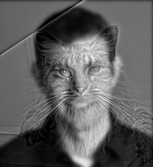
High Frequency: cat
Low Frequency: Derek
sigma for high: 8
sigma for low: 8
ksize: 100
Example 2: Baby and Sea Otter
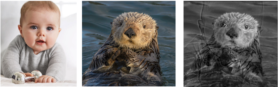 High Frequency: sea otter
Low Frequency: baby
sigma for high: 3
sigma for low: 1
ksize: 100
Example 3: Husky and Cat
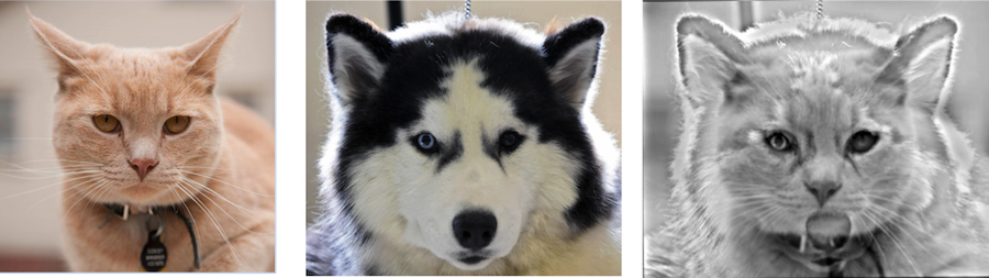
High Frequency: cat
Low Frequency: husky
sigma for high: 6
sigma for low: 1
ksize: 100
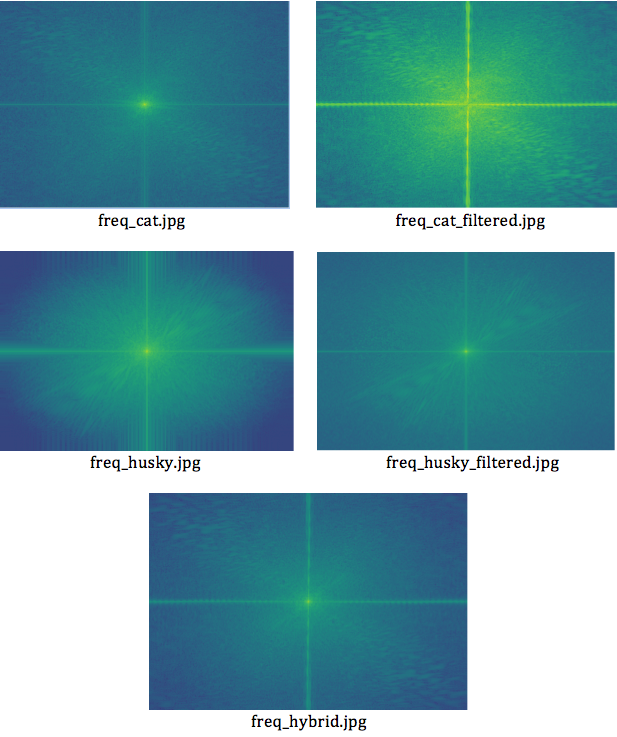
Frequency Analysis:
FAILED EXAMPLE
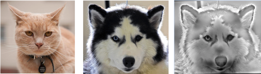
High Frequency: cat
Low Frequency: husky
sigma for high: 8
sigma for low: 8
ksize: 100
The sigma values were chosen wrong so only the husky is shown.
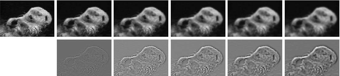
Part 1.3: Gaussian and Laplacian Stacks
The Gaussian and Laplancian Filters created from the parts before is used to creat a Gaussian Stack and a Laplacian Stack.
For Gaussian stack, each sample is downsampled, so the image is more blurred down the stack.
For Laplacian stack, you can think of the image as being a bandpass of the image as each image is current_image - downsampled_img.
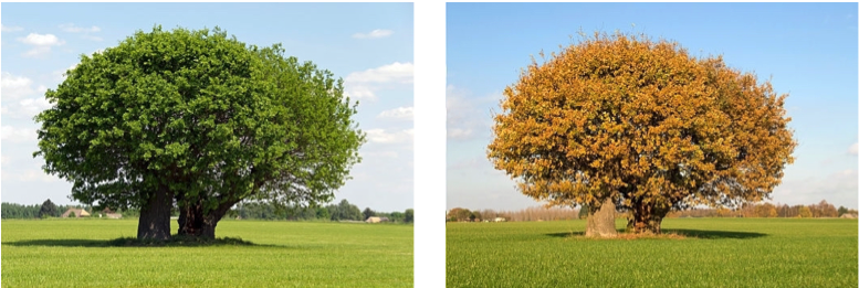
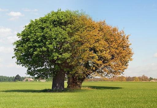
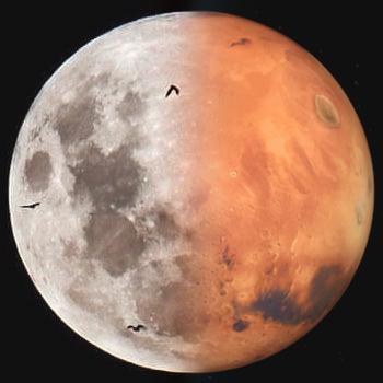
Part 1.4: Multiresolution Blending
In this part, two images are seamlessly blended together using Gaussian blurring of the mask. In each iteration, the Laplacian Stack of the image will be combined with the Gaussian blurred mask, where in the end, the image results in a addition of all the laplacian_stack times the blurred_mask.
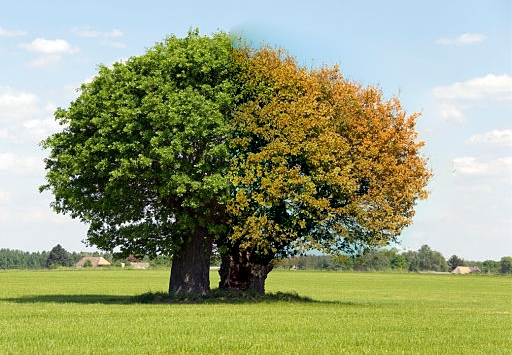
Example 1: Summer and Fall Tree
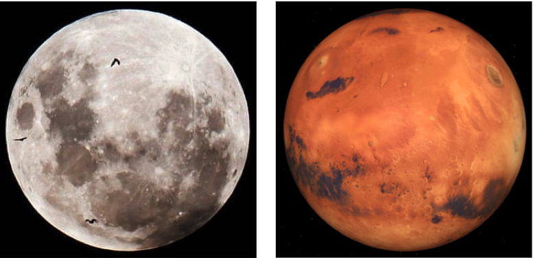
Example 2: Moon and Mars
Part 2: Gradient Domain Fusion
Part 2 is where we use least square to seamlessly blend a source image into a target image. Since the gradient value of the source image and the pixel value of the target value is known, the idea is to alter the pixel value of the source image to match the target image.
The Poisson blending can be done with the equation on the bottom, which is basically an optimization problem.
s: source image
t: target image
v: final source image
The first part of the equation ensures that the gradient within the source image stays the same. This part only applies to the pixels within the mask of the source image.
Meanwhile the second part of the equation ensures that the pixel values at the edge of the mask is same as the pixel values of the target image so that the transition from the source to target is smooth.
By using least square to solve this optimization problem, we can obtain an image that is blended.
Part 2.1 Toy Problem
This part is an intro to the Gradient Domain Fusion where we understand how to set up least squre equation for our purpose. As mentioned before, the goal in this part is to use the gradient information of the source image for blending. Therefore, in this part, we learn how to set up the least squre equation to use the gradient information to reconstruct the original image.
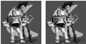
The left is the original toy.png and the right is the image that was created by using the least squre function. Because the gradient and a specific pixel value of the original image is known, the entire image can be reconstructed.
Part 2.2 Poisson Blending
This final part of the project is using least squares to seamlessly blend two images. The equation shown on the top is used to do this.
Example 1: Air Balloon and Blue Sky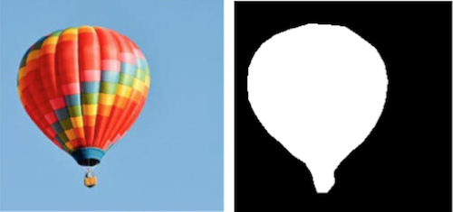
First, a mask is created for the source image, using the masking code provided by Nikhil Shinde. (https://github.com/nikhilushinde/cs194-26_proj3_2.2)
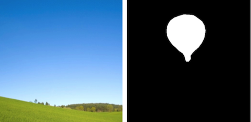
The mask for the target image is also created to know where the source should go in the target.
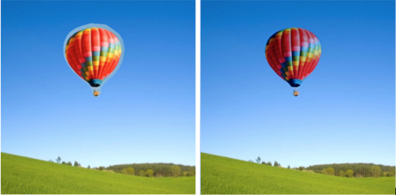
The left image shows how the source image fits into the target without blending. The right image is the one after the Poisson blending is done. You can see that the color of the air balloon in the final image is more blue-ish than the original source image because the color of the sky was different. However, the blending is done pretty well.
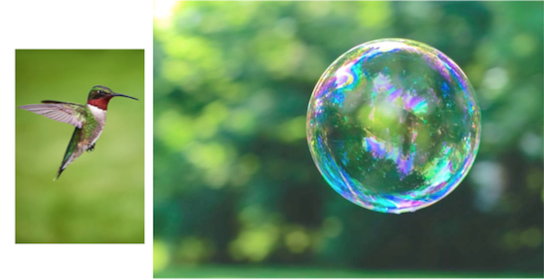
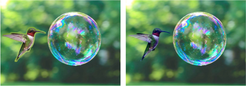
Example 2: Hummingbird and Bubble
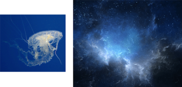
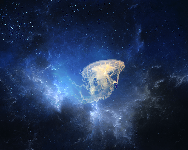
Example 3: Jellyfish and Night Sky
Example 4: Earth and Snow Globe
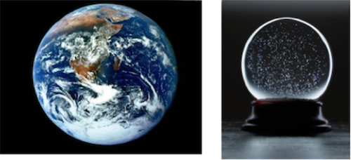
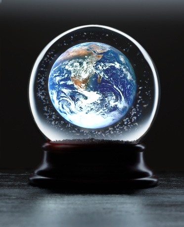
FAILED EXAMPLE
Example 5: Sea Otter and Green Tea
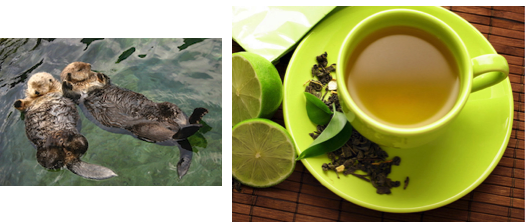
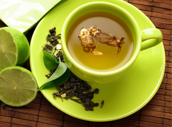
You can see that because the color of the water from source image was very different from the color of the tea from the target image, the final result is not very smooth. Also, since the source image had water waves shown while the green tea is smooth, the transition is noticable.
Comparing Poisson Blending and Laplacian Pyramid Blending
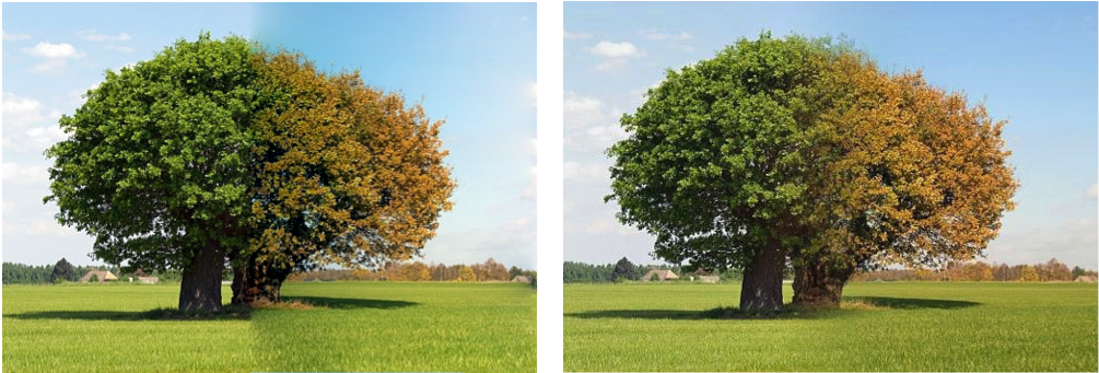
The left image is Poisson Blending and the right is Laplacian Pyramid Blending.
First of all, you can notice that the mask for Poisson Blending is not perfect because for this particular image, using a 1/2 mask is easier than the arbitrary mask that Poisson blending uses.
Another difference is that the sky color gradually changes for Poisson blending while for Laplacian Pyramid Blending, the very left part of the image is same as the original because it is outside of the blending mask.
The disadvantage of the Poisson Blending is that the color of the original image is not kept if the target color is overpowering. Above in an example of Poisson Blending where only the right side of the tree is masked with the fall tree, instead of the entire half of the image being the mask. You can see that the green affects the yellow a lot. However, the rest of the target image is untouched and the resulting image blends in pretty well.
In conclusion, when the source image color is similar to the target, then Poisson Blending works very well. However, when their colors are very different, this affects the source image color a lot, which is not nice for the resulting image.
Last Edit: 10/3/2018