Fall 2018 CS194-26 Project3
Jieming Wei
1.1: Warmup
Sharpening image with unsharp masking
I used the gaussian filter of size 19 and sigma 4 to generate the gaussian blurred image. Then, I add the blur image to the original one with alpha set to 2 and normalize the total brightness to get the final result.
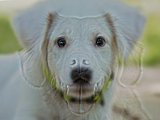
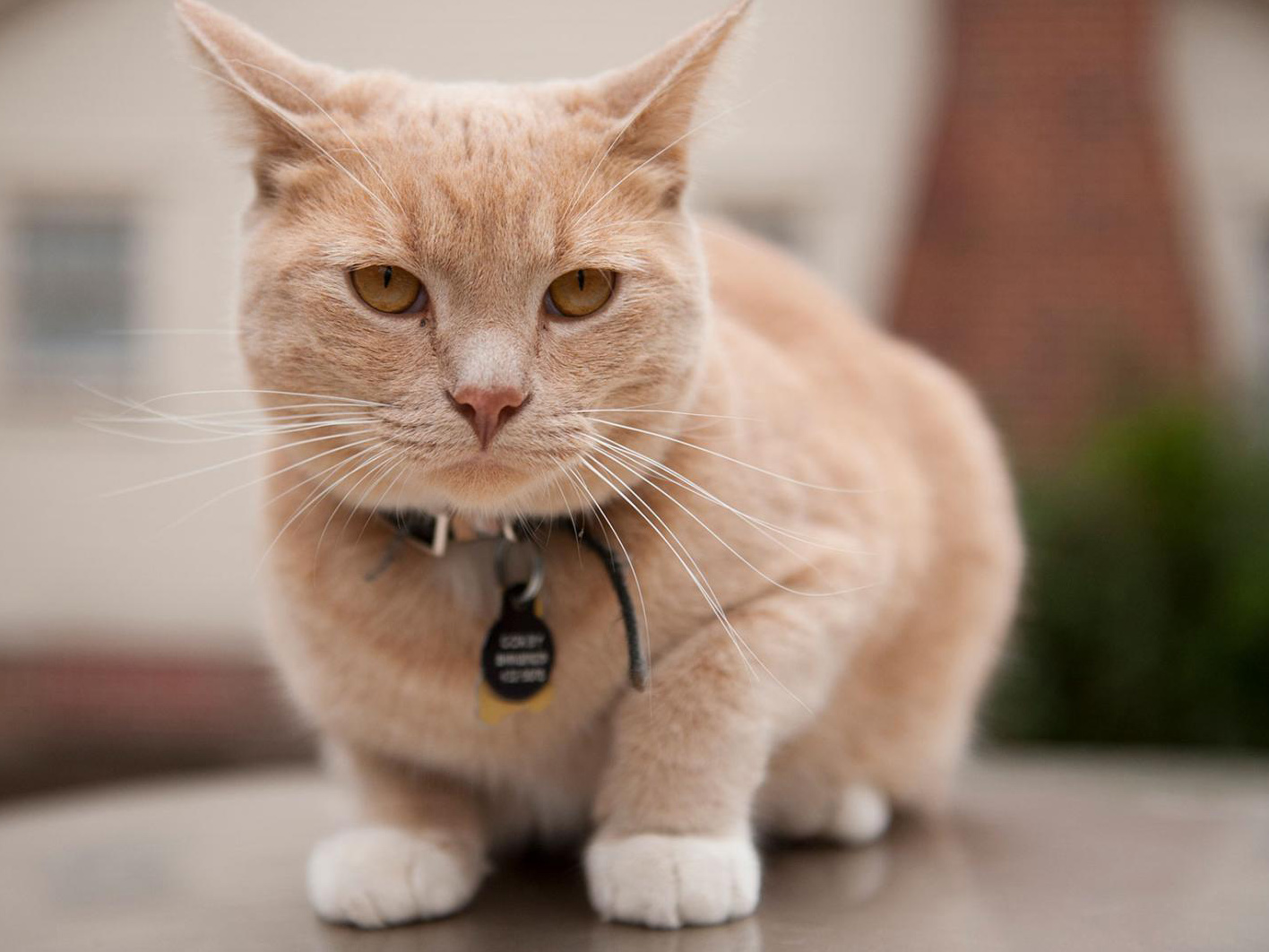
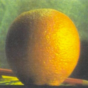
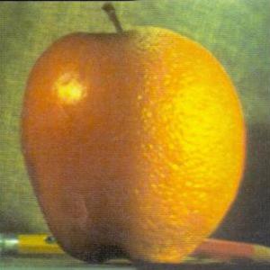
1.2: Hybrid Images
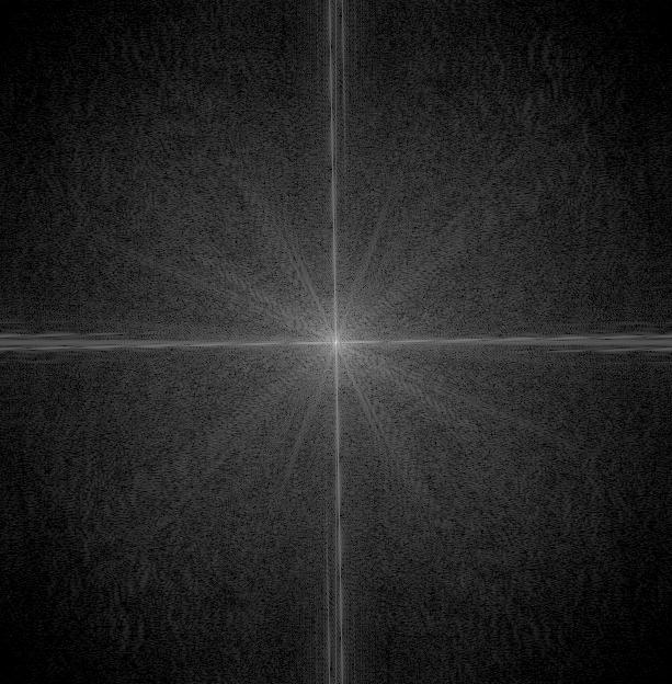
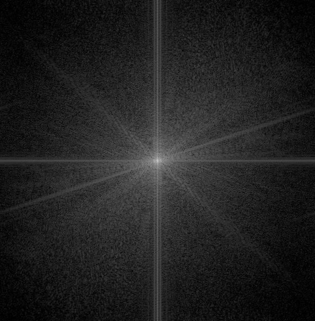
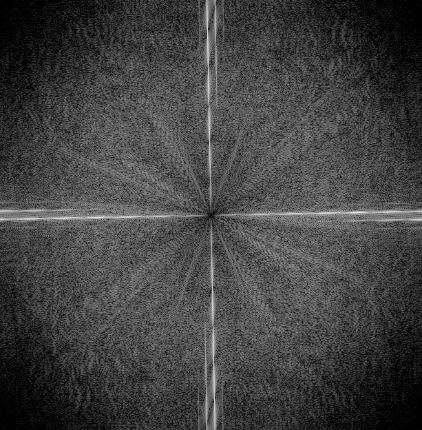
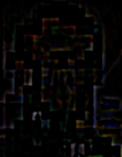
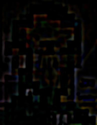
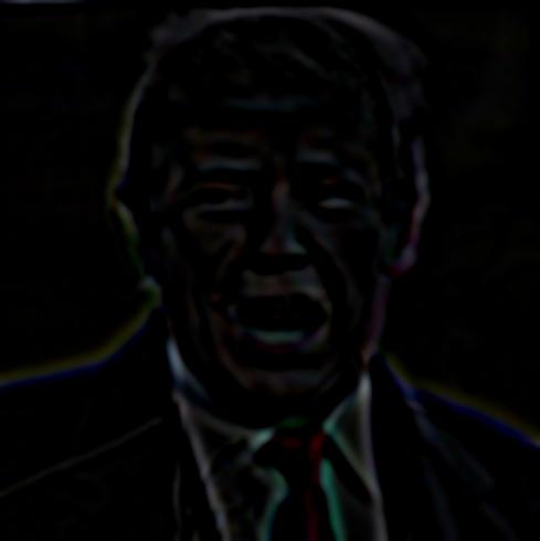
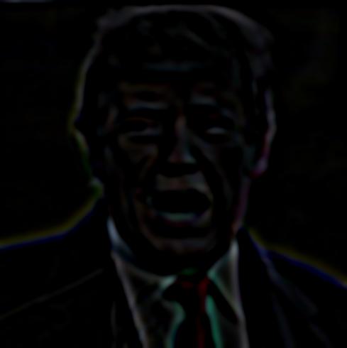
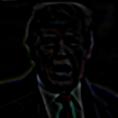
Hybrid images and the Fourier analysis
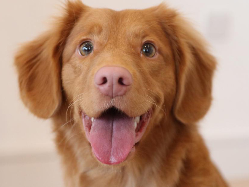
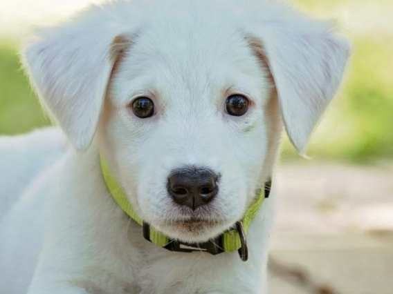
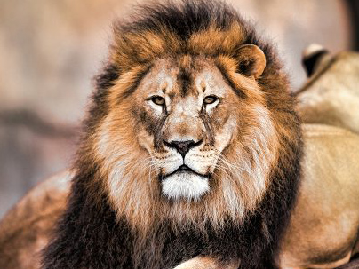
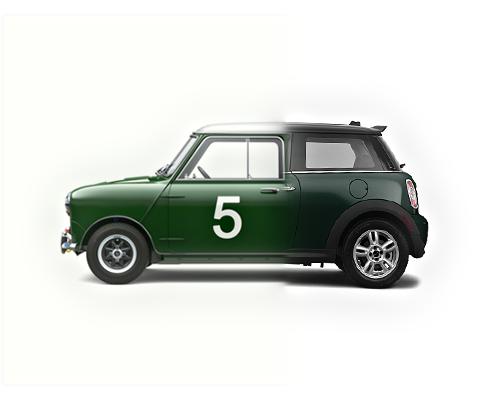
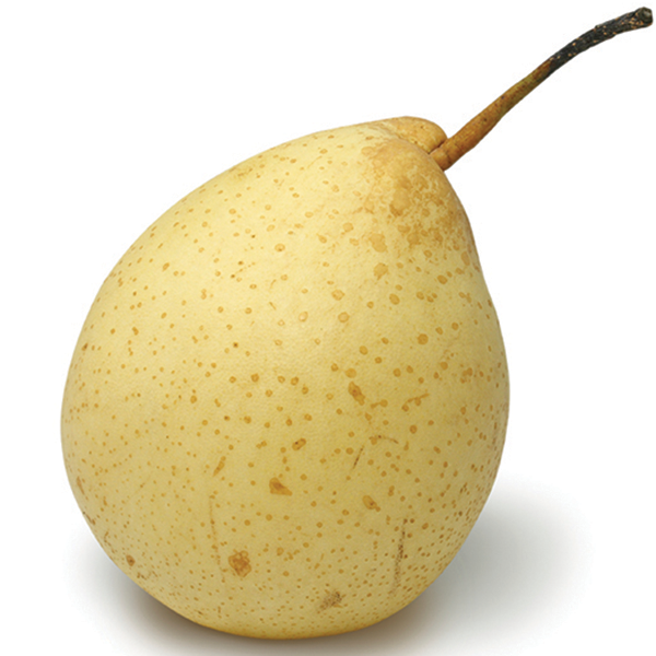
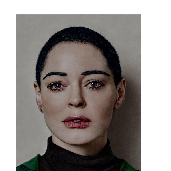
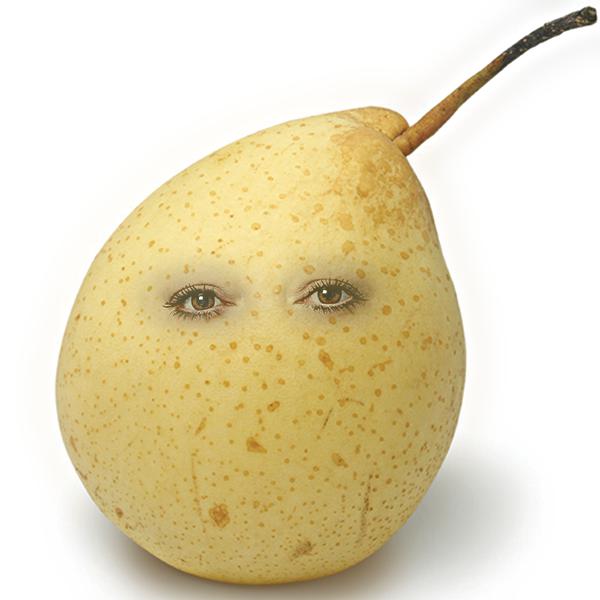
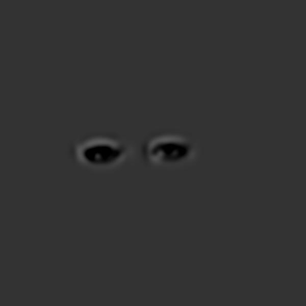
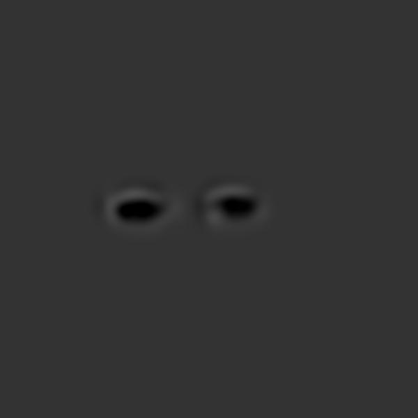
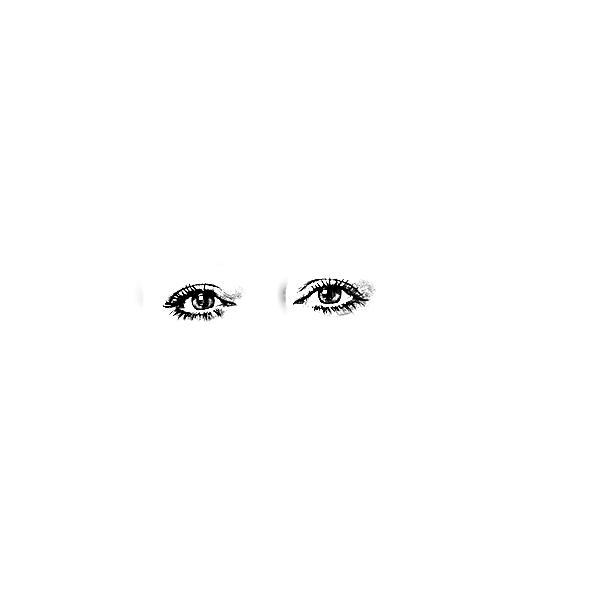
These hybrid images are generated by weighted averaging two images. One of them is a image get filtered by high pass filter and another one filtered by low pass filter. The low pass filter is a gaussian filter. The high pass filter is a one subtracting gaussian filter by the original image. I used sigma value of 3 for the high pass filter and sigma value of 13 for the low pass filter for the following images.
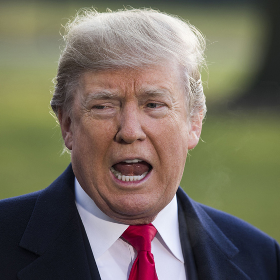

Fourier analysis
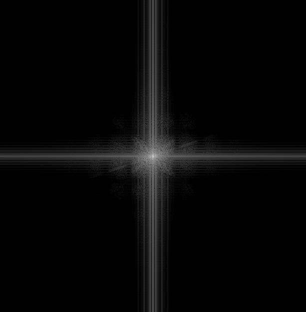
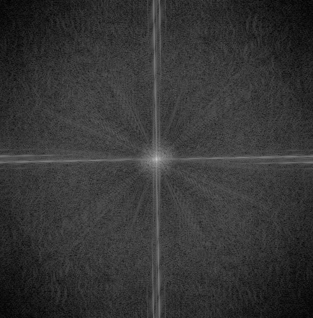
More result
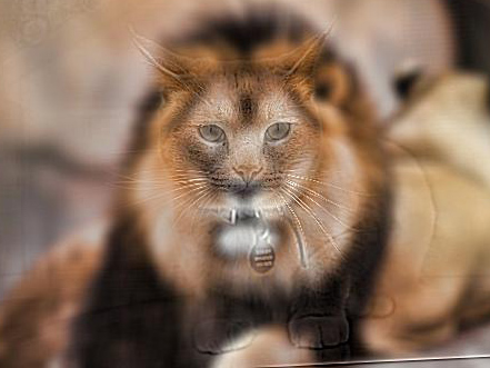
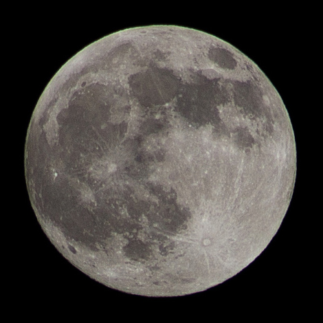
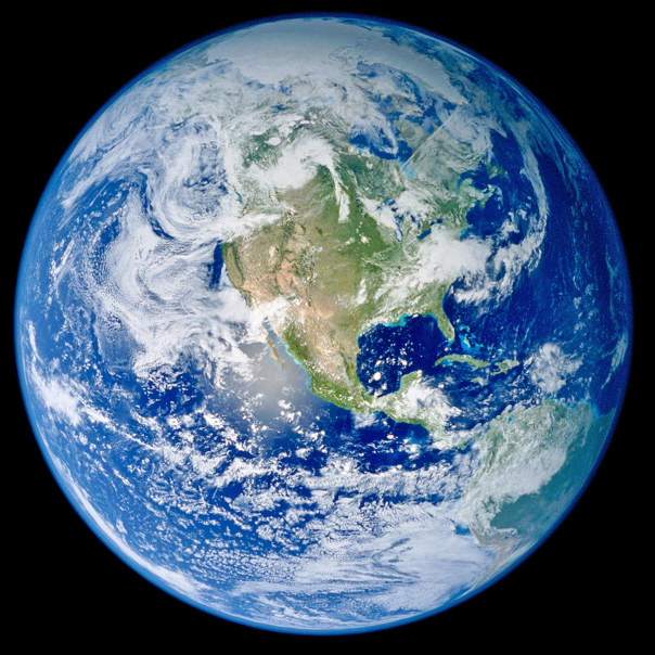
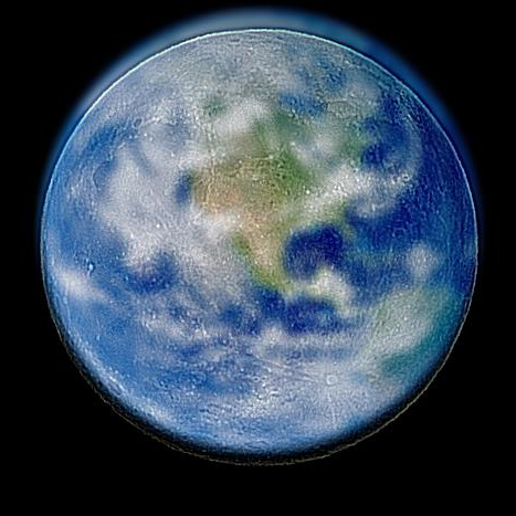
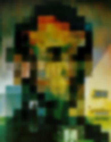
failure result
The case of earth and moon failed because the pattern on the moon is not obvious enough and get masked out by the pattern on earth.
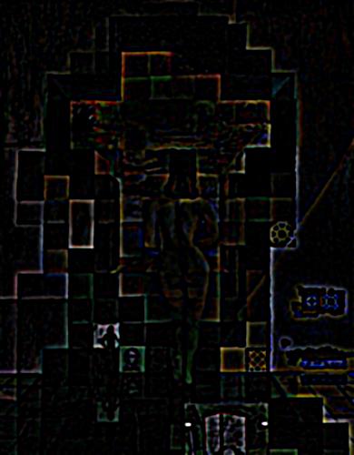
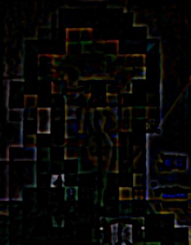
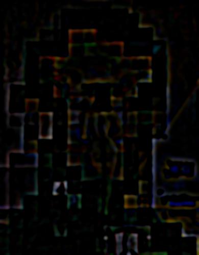
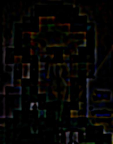
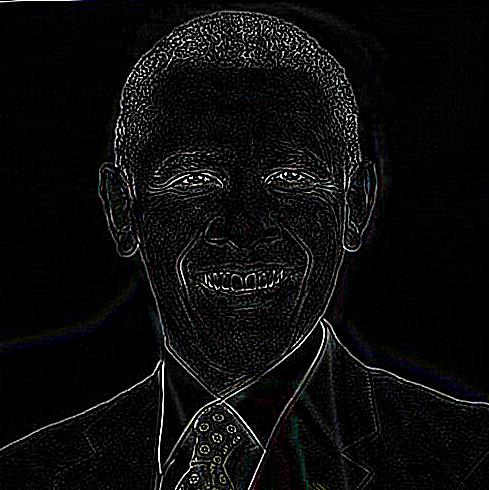
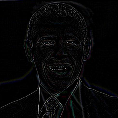
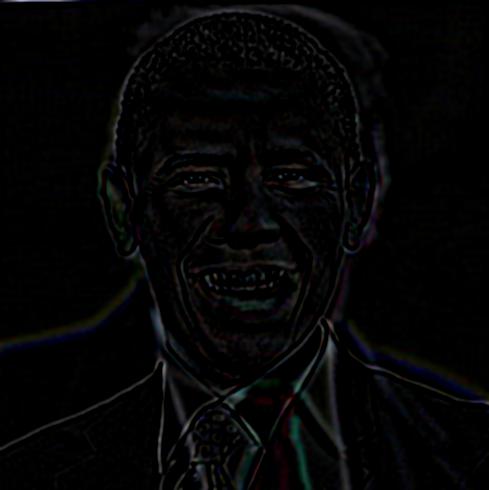
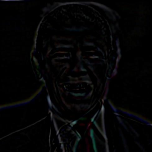
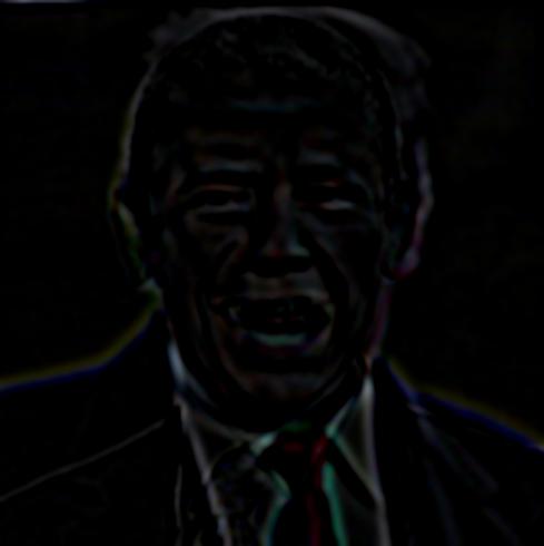
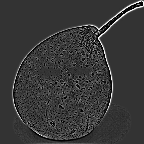
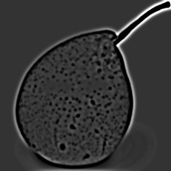
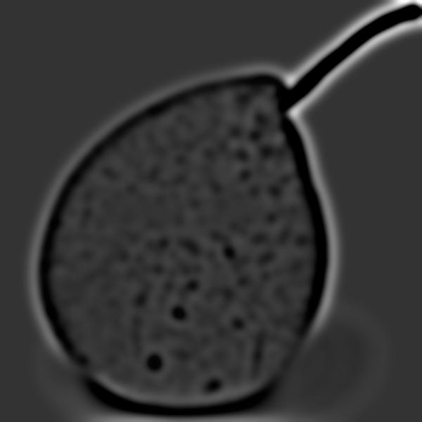
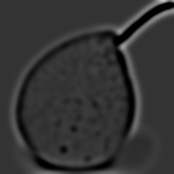
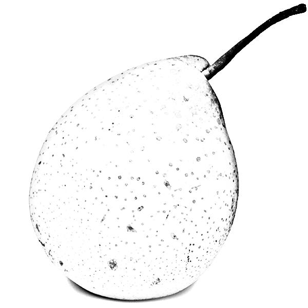
1.3: Gaussian and Laplacian Stacks
Gaussian stacks is generated by having the original image get filtered by gaussian filter with different sigma. For the following image, I used sigma values of 4,6,8,10,12,14,16,18. Laplacian stacks is generated by subtrating image of each level of gaussian stack from the previous level. I have increased the brightnees of each image in laplacian stack so it is more obvious.
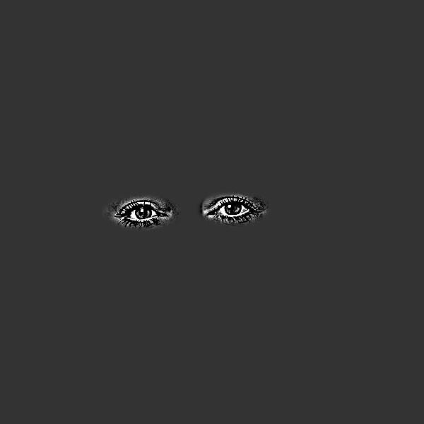
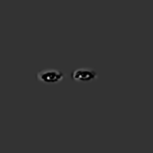
Lincoln Gaussian stack


Lincoln Laplacian stack


part 1.2 Gaussian stack


part 1.2 Laplacian stack
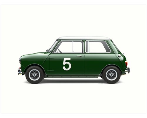
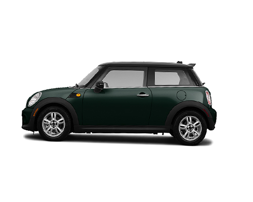
1.4: Multiresolution Blending
In multiresolution blending, I blended two images by first decomposing two images into different frequency domains respectively. Then I combine images with same frequency level and finally add them up together. Note the higher frequency image have more clarity and lower frequency image get blurred by gaussian filter.


Laplacian stack decomposition
Part2
Description
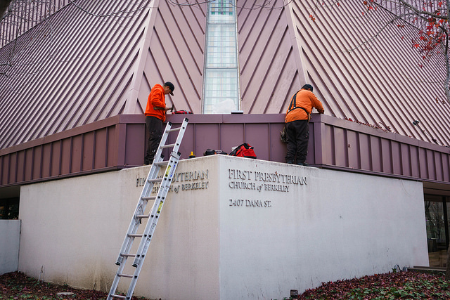
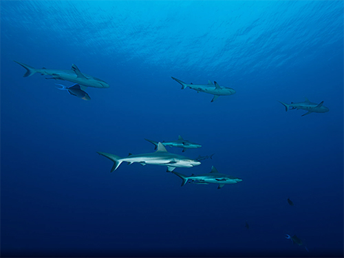
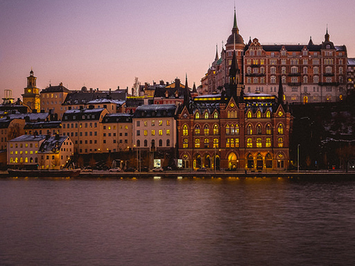
In this part of the project, we are implementing poisson blending and a related toy problem. The purpose of the algorithm is to blend a portion of a picture into another picture. The problem of direct copy is that not only will we get a sharp edge but the color tune of source image and target image could be entirely different. In poisson blending, we try to solve this problem by consider all the target pixals as unknown variables and solve an optimization function on them.  Referenced from cs194-26 proj3 spec, in the first part of the optimization function, we want the gradient of target portion to be as similar as the original portion of the source image. In the second part, for all pixal around the target mask, we want to the gradient to be similar as the arund pixal of target image. In this way, we won't see any sharp edge and the pattern in the output will almost match the target pattern. Besides, the color will be similar.
Toy problem
In the toy problem, we want to recontruct the original picture by solving an optimization function where we want the gradient of target image almost match the gradient of the source image. Besides, we want the upper left most pixal to almost have the same value. Under these two constraints, we can techinically get the same result as the original one.

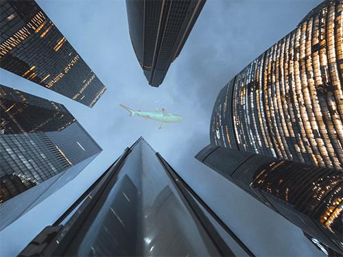
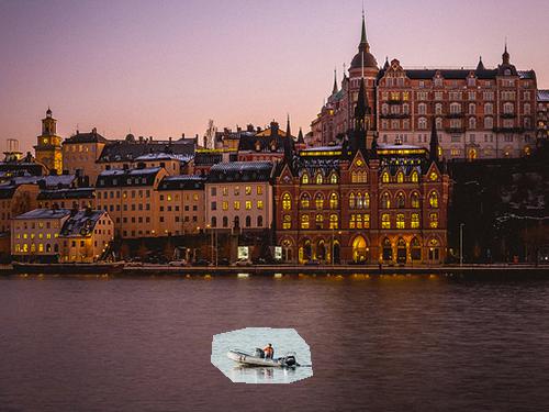
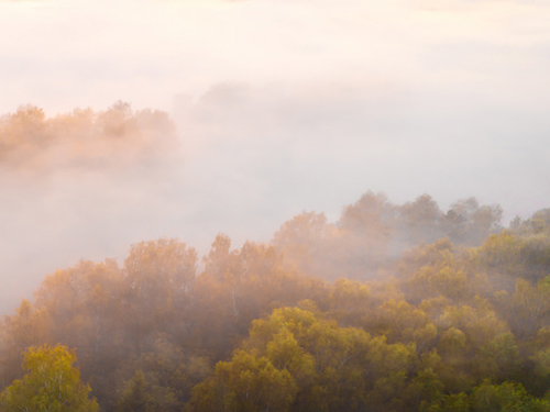
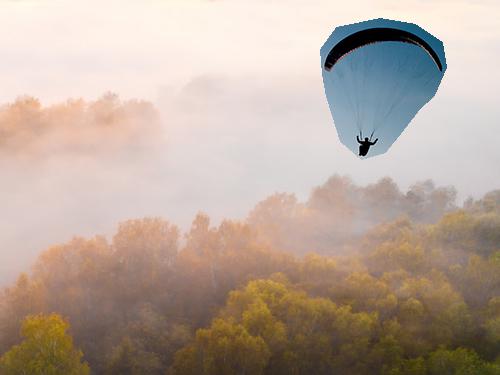
Poisson Blending Results
Procedure
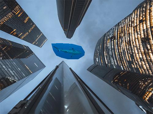
I create mask for both target and source image, which are pictures with only white and black pixals. Then I calculated the row and column offset between these two masks. The offset will be used to find the corresponding source pixal for each target pixal. When constructing the matrix A and vector b, I just follow the optimization function. I used a helper function to convert a two dimension index to a one dimension index. Since the target portion is a irregular mask, I used a dictionary to store the one-to-one mapping from 2 dimension index to the actual row number in matrix A. After the least square gets solved, I copied back the result to the result image according to the mapping I created before. I optimized the performance by making sure all the rows and columns in matrix A have non-zero number, therefore, reducing the matrix size.

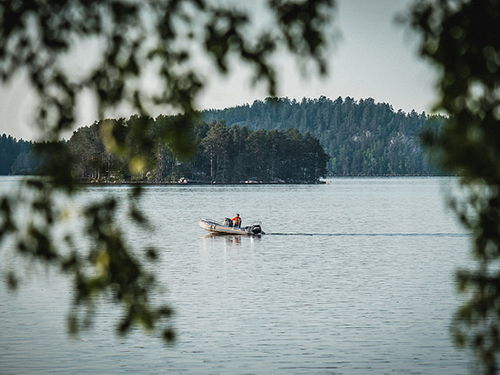
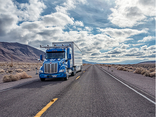
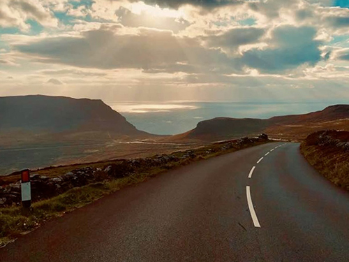
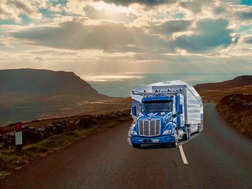
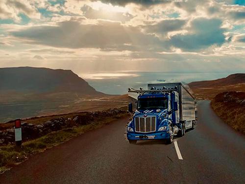
Poisson Blending Failed Results
This example fail for two reasons. First, the angel of the truck is not well matched between the source image and target image. Second, the truck cannot be easily seperated from the background. As result, there are still some wired partten around the truck in the final result.
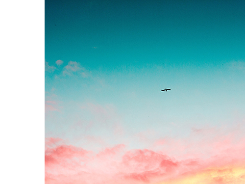
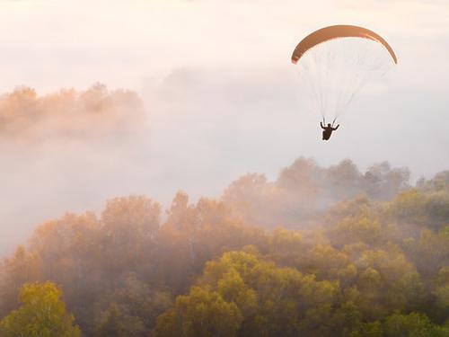
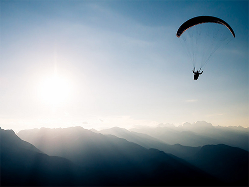
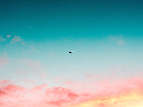
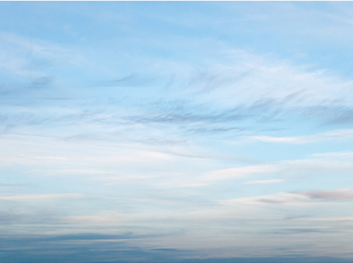
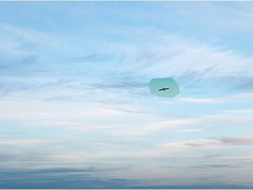
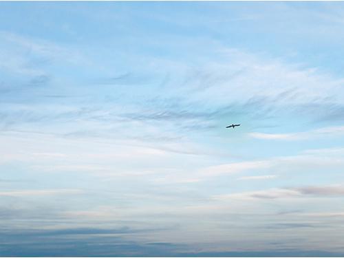
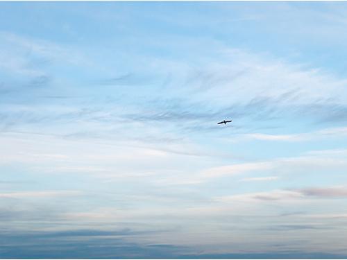
Laplacian pyramid, Poisson Image, Mixed graident comparison
For this case, the mixed gradient works the best. The reason is that mixed gradient take both source and target image into consideration and choose one with larger gradient as a reference. In this way, it successfully captured both the bird from the source image and the cloud texture from the target image. We should almost never use direct copy. We can only use Laplacian pyramid blending when the color tenperature of both image is similar, which does not apply for this case. We can use Poisson Image Blending when the edge of mask from both target and source image have similar pattern. For example, it works well with clear sky and water. However, it does not work well for this bird case because the cloud condition is different for source and target. The most important thing learned from this project is the relativity is more important than the actial value.

Bells & Whistles
1. I implemented hybrid image with colors. It works good with both have colors
2. I implemented multiresolution blending with colors.
3. I implemented Mixed Gradients and the result is shown at the comparison section in part 2.