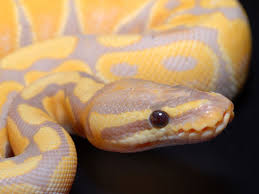
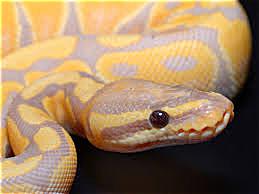
For the first part of this project, I applied the unsharp produce to sharpen the
following image of a banana snake.
First, apply a gaussian filter to smooth the image (achieved by convolving).
Subtract the smoothed image from the original image to obtain the
high frequencies of the image.
Add back some porition of the high frequencies to the original image.
The fraction added by is controlled by a parameter alpha.
Using a 7x7 gaussian filter with sigma = 2 and a choice of alpha = 0.9 achieves the following result.
Original imageSharpened image.
For our reptilian friend, it appears that mostly it's scales are composed of high frequencies.
These are noticably more contrasted in the sharpened image.
Part 1.2 - Hybrid Images
In the previous part, we took the high frequenices of an image and increased them to sharpen an image. But what would happen if we decided
to take these high frequences and add them to the low frequencies of another image?
We know high frequency tends to dominate perception when it is available,
but, at a distance, only the low frequency (smooth) part of the signal can be seen. By combininng different frequency ranges
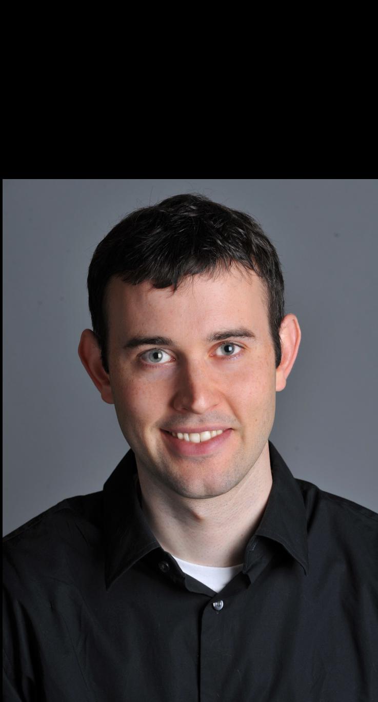
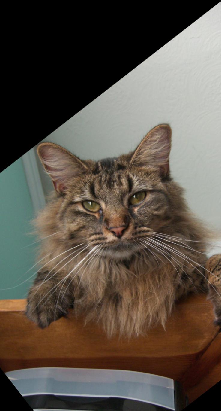
of different images, we create hybrid images. For example, below is what we get if we combine the low frequencies of Nutmeg the cat and of Derek:
Image 1: Nutmeg
+
Image 2: Derek
=
Hybrid
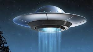
Below are two other examples of hybrid images:
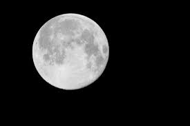
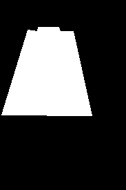
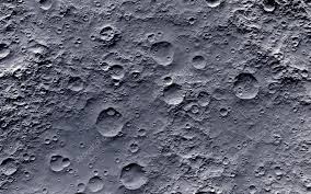
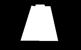
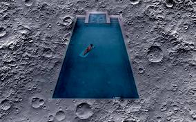
Image 1: Ufo
+
Image 2: Moon
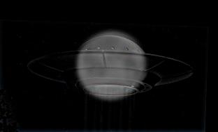
=
Hybrid
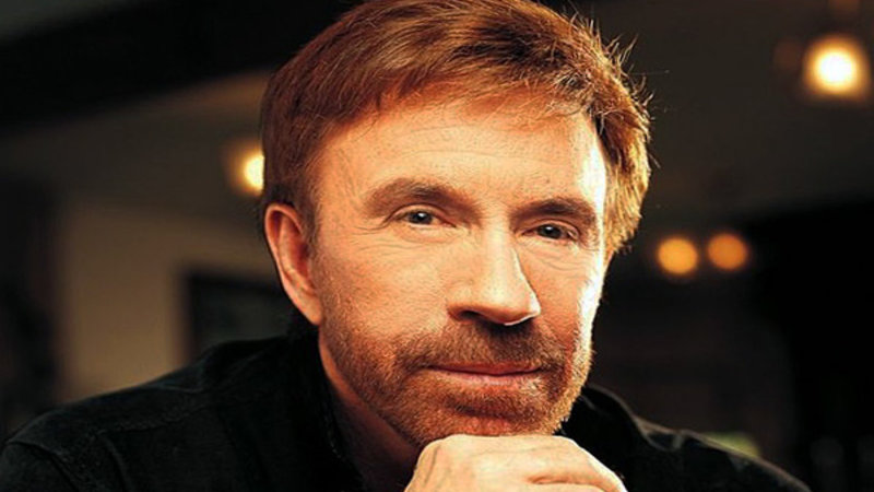
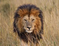
Image 1: Chuck Norris
+
Image 2: Lion
=
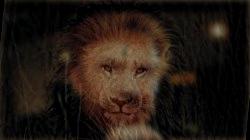
Hybrid
The Chuck-lion hybrid lion turned out decently well, but the ufo-moon hybrid really did not.
Fourier Analysis
All of the images were filtered with a 13x13 gaussian filter with sigma = 4. By playing around with sigma, change cutoff freqency.
Only requencies below the cutoff frequency retained for one image, and only frequences above the cutoff frequency are retained for the other image.
These two sets of frequencies are then averaged to produce the hybrid image.
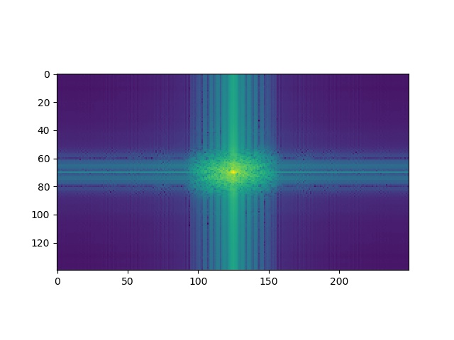
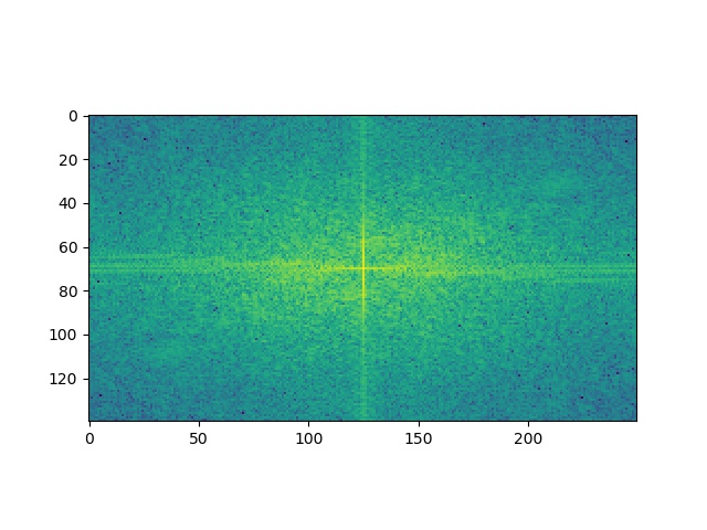
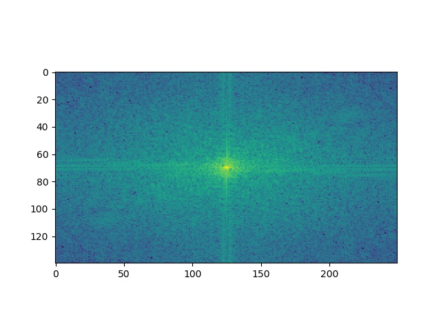
We can visualize this process by casting the problem into the frequency domain via FFT for the Derek-Nutmeg image:
Low Frequencies - Chuck NorrisHigh Frequencies - Lion Hybrid Frequencies
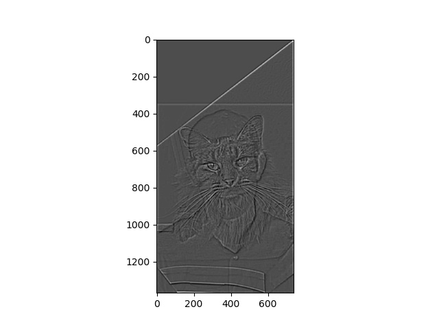
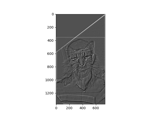
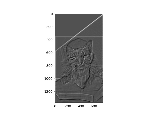
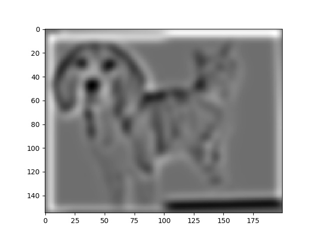
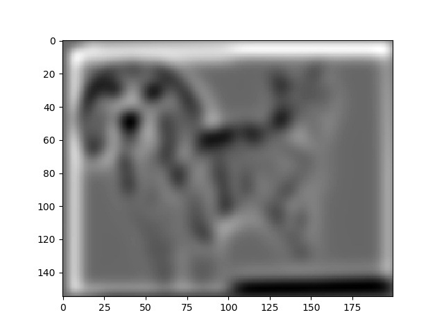
Part 1.3 - Gaussian and Laplacian Stacks
A Gaussian Stack is a series of images we get by applying a gaussian filter to an image and repeatedly applying
the same filter to the resulting filtered images.
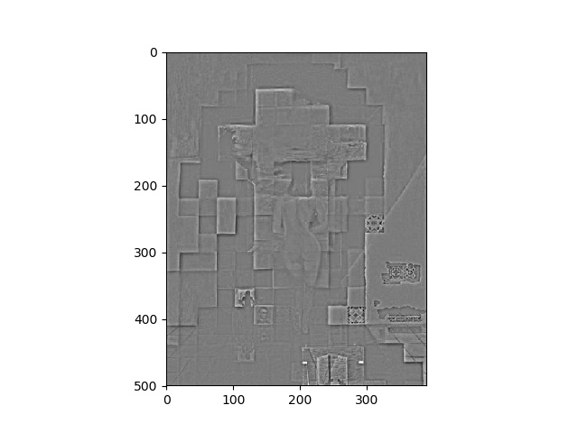
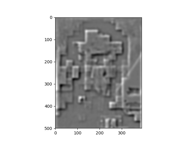
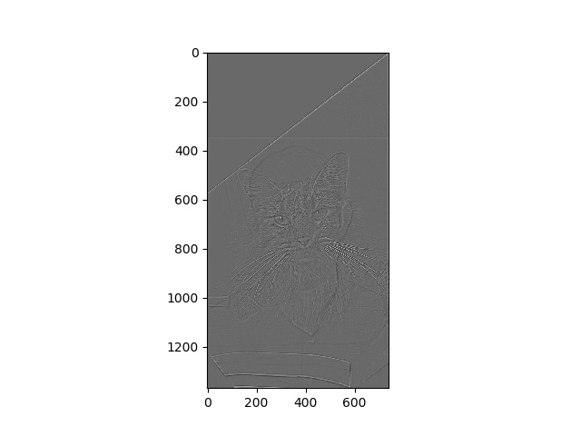
A Laplacian Stack is a series of images we get by subtracting sucessive pairs of images of the gaussian stack. The first image of the
laplacian stack is the original image subtracted from the one-filtered gaussian stack image.
Instead of just creating low and high frequency poritions of images, the process of creating a Laplacian stack creates a series of band-passed images.
Band-passed images have a low and high cutoff frequency, and in our case, these laplacian frequency bands are distinct from each other.
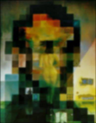
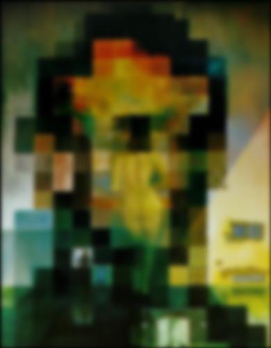
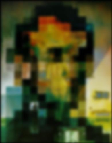
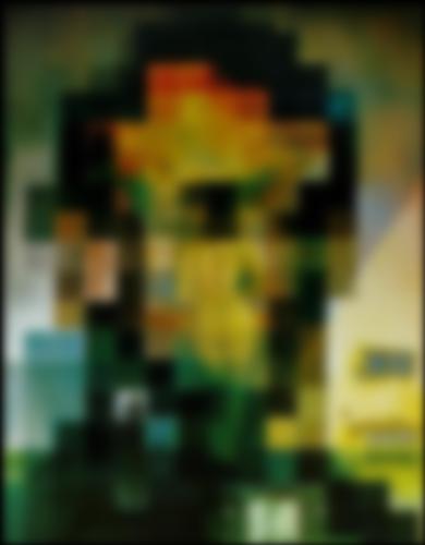
Below I display a 6 layer Gaussian stack and Laplacian stack for the Salvador Dali painting of Lincoln and Gala and the Derek-Nutmeg hybrid:
Part 1.4 - Multiresolution Blending
If we attempt to combine two images together naively the image spile created is too jagged. To get a smooth spile, we can use the method described
in the Multiresolution Blending paper by Burt and Adelson (1983). The idea is that instead of simply blending everything at once, we blend the images
at different resolutions to create a smoother spile. To do this, I created a Laplacian Stack LA for the first image, a Laplcian Stack LB for the second
image, and a Gaussian Stack for the mask, GR. At each level of the stack, a stepwise function with the respective blurred mask as weights to combines
the two slices:
Finally, the new Laplacian Stack LS is summed together along with the bottom stack of the Gaussian Pyramid for each pyramid to reconstruct a new, seemless image. For all of the following images,
I used a 12x12 Gaussian filter with sigma=3 to create the stacks, and each stack had 8 layers each.
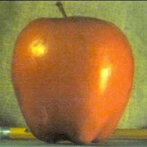
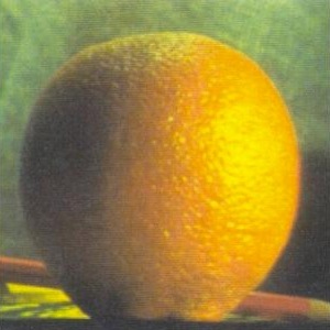
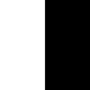
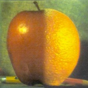
Example 1: Orapple
Image oneImage twoBinary MaskBlended Image
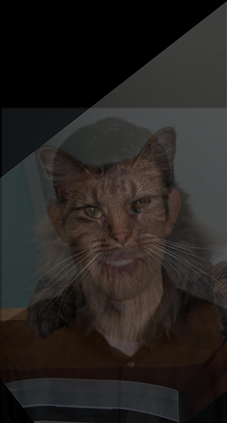
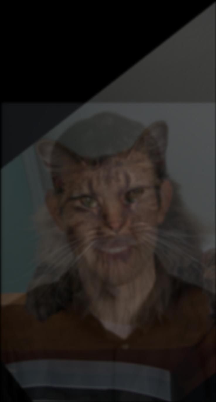
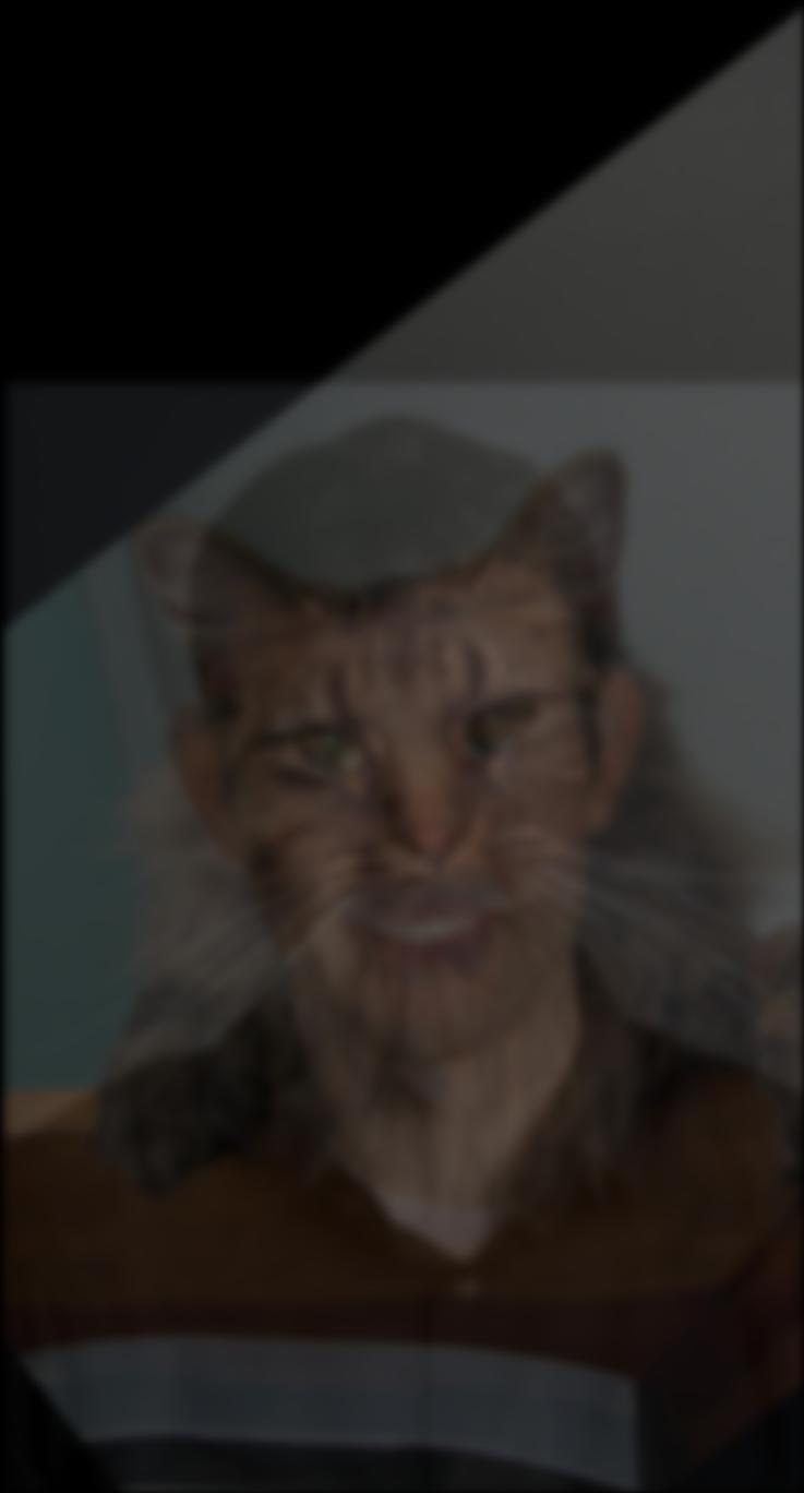
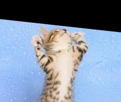
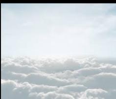
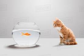
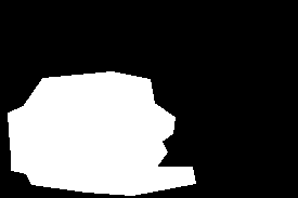
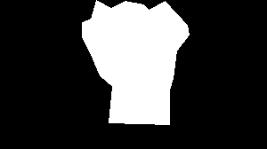
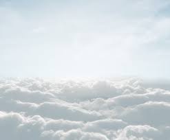
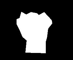
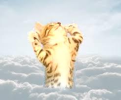
Example 2: Sky kitten
I envisioned a giant cat rising from the clouds when creating this image. However, due to the blue background of
the cat picture didn't mix well with the mostly white cloud picture.
Image oneImage twoBinary MaskBlended Image
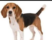
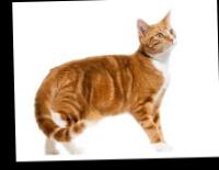
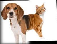
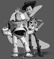
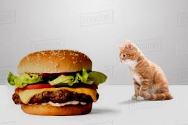
Example 3: Catdog
This is the image I am most proud of. Based of th old Nickelodeon cartoon, I seemed a cat onto the end of a dog. This one
turned out quite nice, despite only utilizing a binary mask.
Image oneImage twoBinary MaskBlended Image
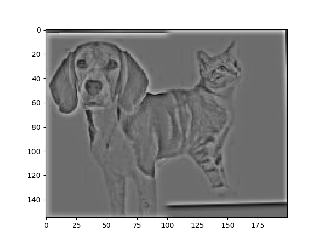
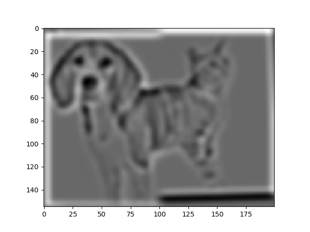
Below I display the itermediate Laplacian Stack LS that are combined together with the
lowest Gaussian Stack level to to create the blended image:
Part 2 - Gradient Domain Processing
Part 2.1 - Toy Example
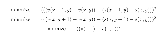
For this part, we take the original image, compute its gradients, and use them to reconstruct the original image. We can accomplish this by
solving for v subject to the following constraints:
In the above image, s is the source image and v is the target image. The first constraint ensures that the x-grandients of v are close to
the x-grandients of s. The second constraint ensures that the y-grandients of v are close to
the y-grandients of s. And the third constraint ensures the the top two corners are the same color. In this problem, the pixels of v are the variables
we are solving for. We solve for v using a least squares solver. Below show the original image and the image reconstructed from the gradients (v):
Original ImageReconstructed Image
Part 2.2 - Poisson Blending
We can take the idea of gradient domain processing and use it for blending. To do this, we take a source region in the source image and a target
region in the target image, which we can represent with two image masks. We want to move the pixels in the source region into the target region seemlessly.
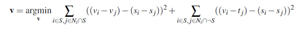
To do this, try to solve for v in the following least squares problem:
In this problem, Ni is the 4-set of neighbors of pixel i of the source region, s is the source region, and t is the target image.
The first half of the blending constraint ensures the the differences between the pixels in source region and result (gradients) are as close as possible.
The second half of the blending constraint ensures that differences across the boundaries of the source region and the new region are similiar to the target image outside
the target region and similiar to the source image inside the region. Assuming there are n pixels in the source image, we can represent this problem as a system of 4n equations (unknown)
with n unknowns, whose solution (found using python) produces a set of new pixels v that we copy into the target region. This is poisson blending in its entirety.
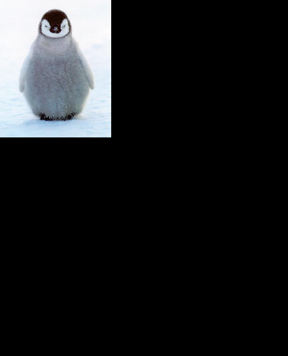
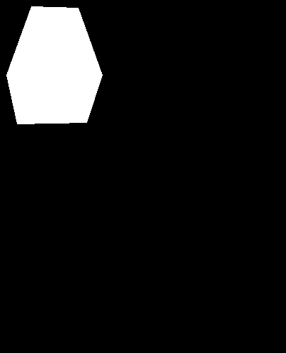
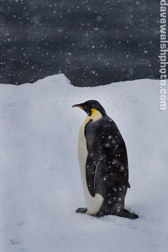
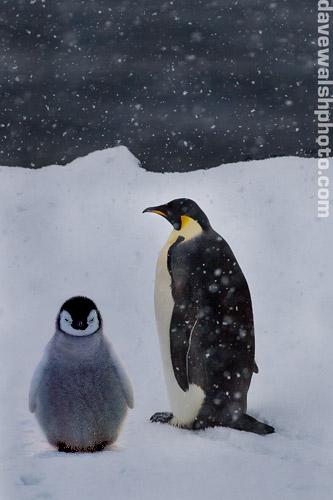
Penguins
Using Poisson Blending, we can re-unite the penguins that have been lost in our sample image folder:
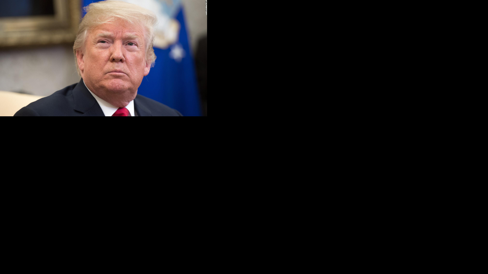
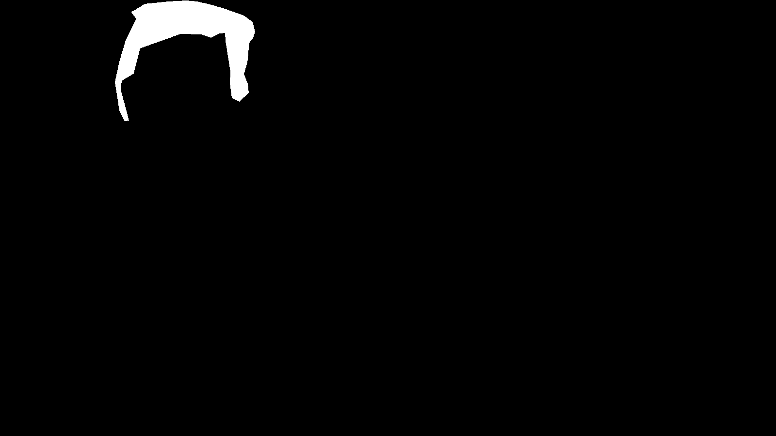
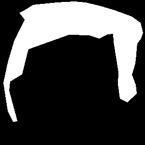
Second: Source ImageSource Mask Target ImageTarget MaskBlended image
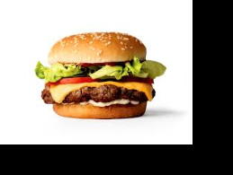
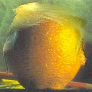
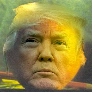
Using Poisson Blending to put Donald Trump's hair on an orange works decently well. However, when we try to put his face on the
orange, we get less than stellar results. The lighting in the orange picture produces a weird color effect that persists in the blending image.
It appears the lighting causes the gradient of the target image (outside boundary of target region) that are alot differernt than anything from the source image.
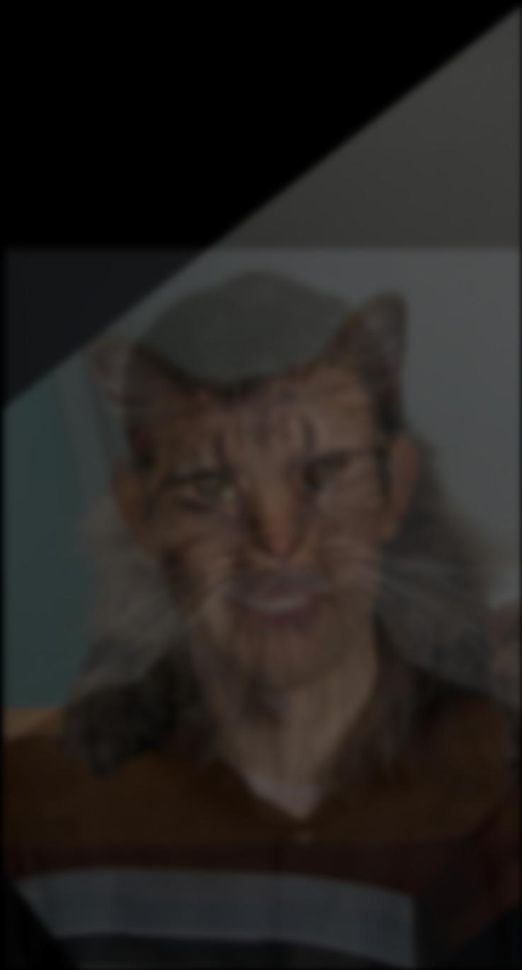
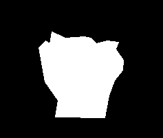
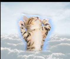
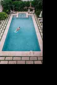
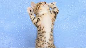
Kitten in the clouds
Since the Multiresolution blending failed for creating a kitten coming out of some clouds in Part 1.4, I decided to see if Poisson Blending would do a better job because there were significantly
different boundary colors. Although the kitten is a different color, Poisson blending handled the difference in background colors really well, producing
and almost seemless stiching.