Computer Science 194-26: Image Manipulation and Computational Photography
Project 3: Fun with Frequencies and Gradients!
Ari Pickar
Part 1.1:
In the first part of this project, I were exploring what happens when you play around with the frequencies of an image. To create a hybrid image, I took an image, convolved it with a guassian kernel, and then added the difference between the original image and the convolved image (multiplied by a constant, in this case 7) back to the original.
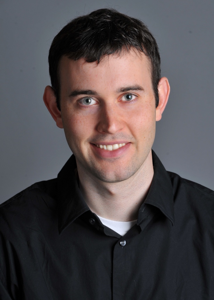
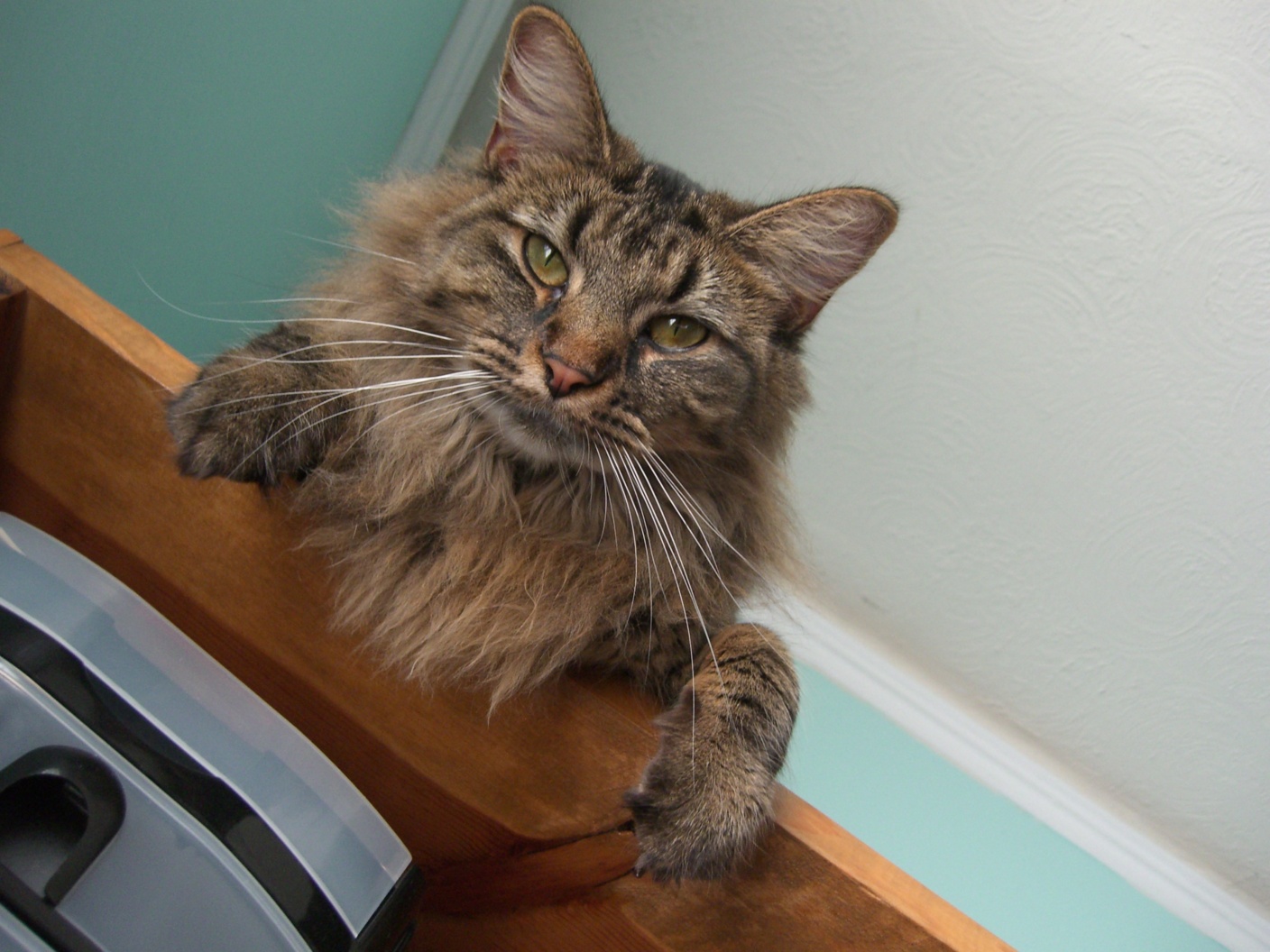
Original Image:
Sharpened Image:

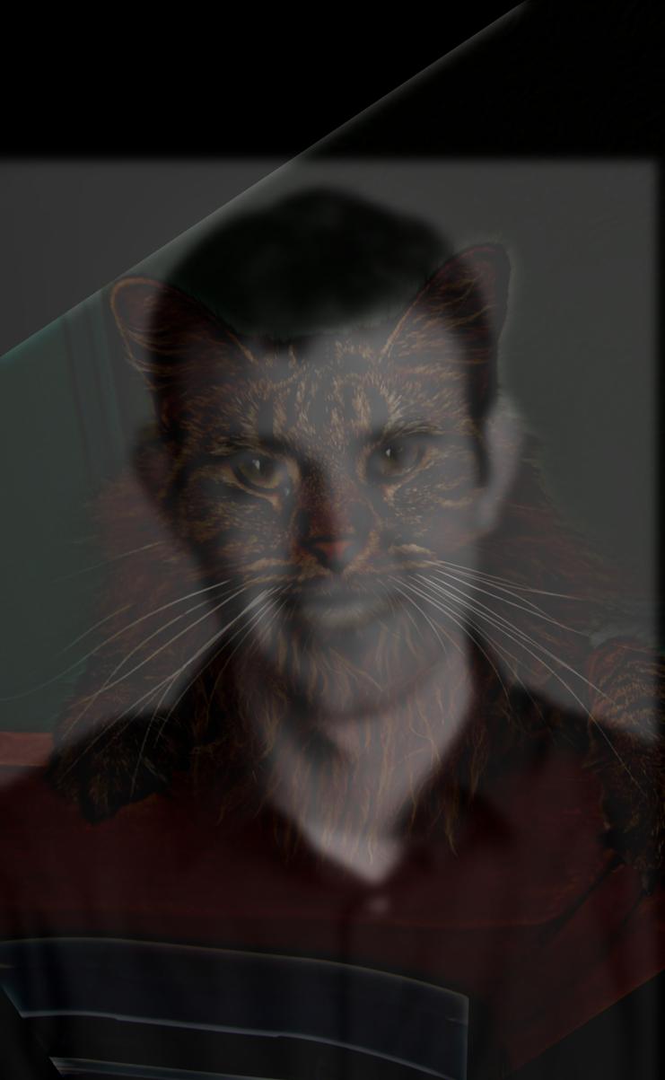
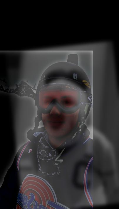
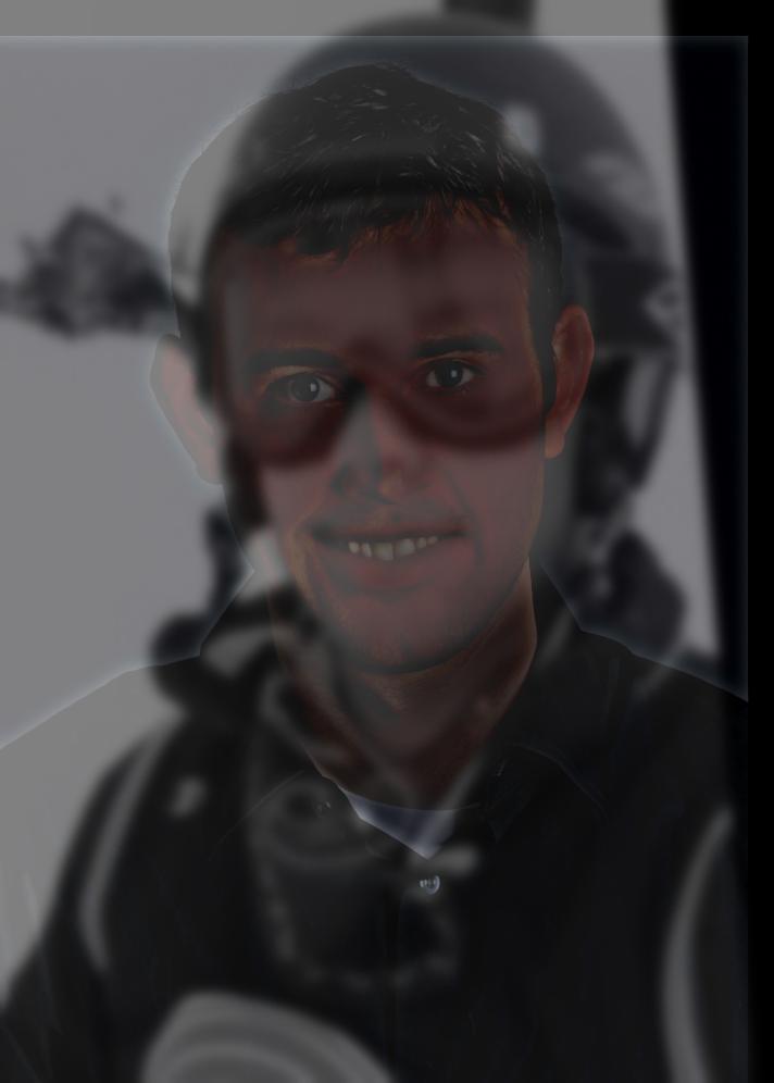
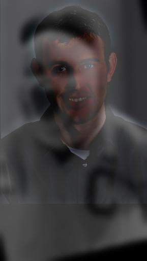
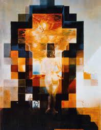
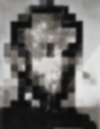
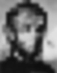
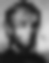
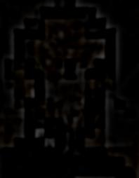
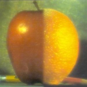
1.2 Hybrid Images:
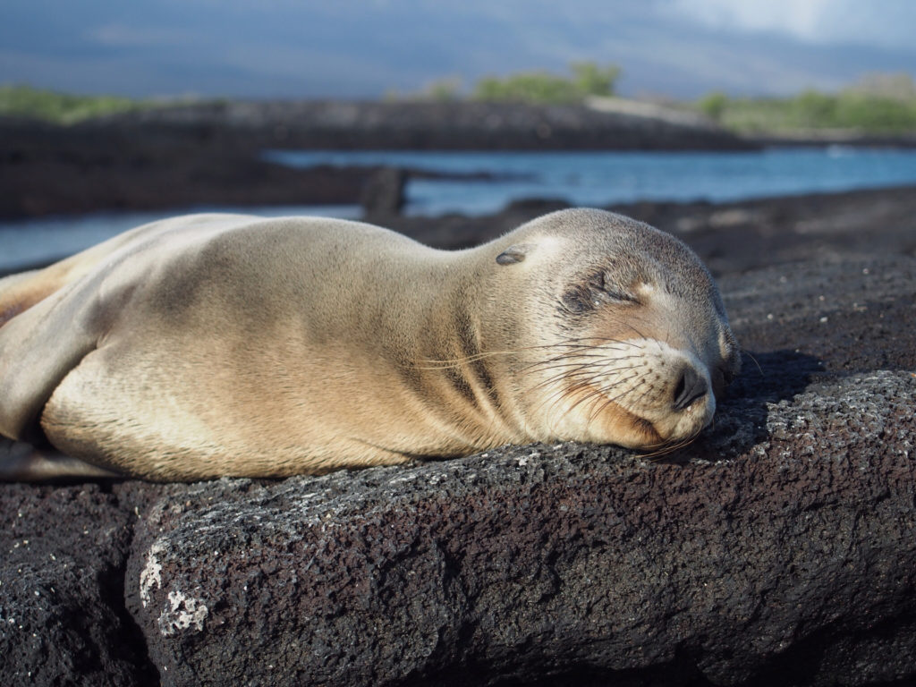
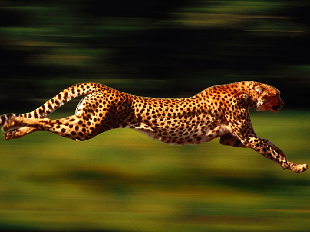
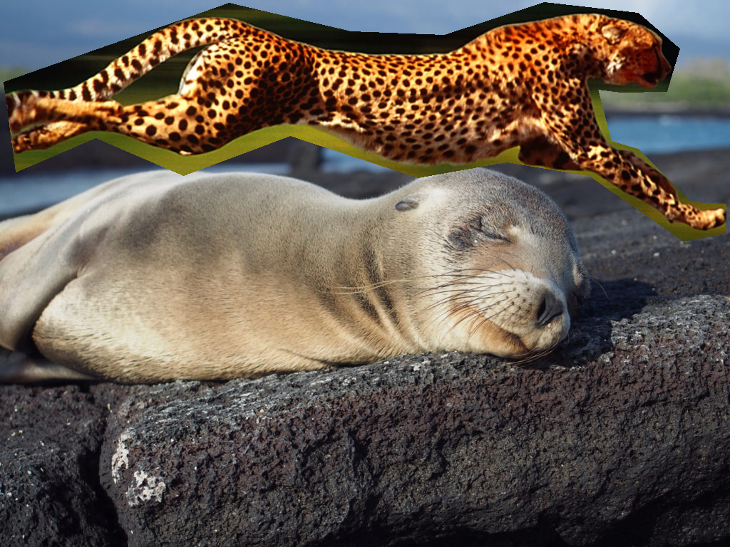
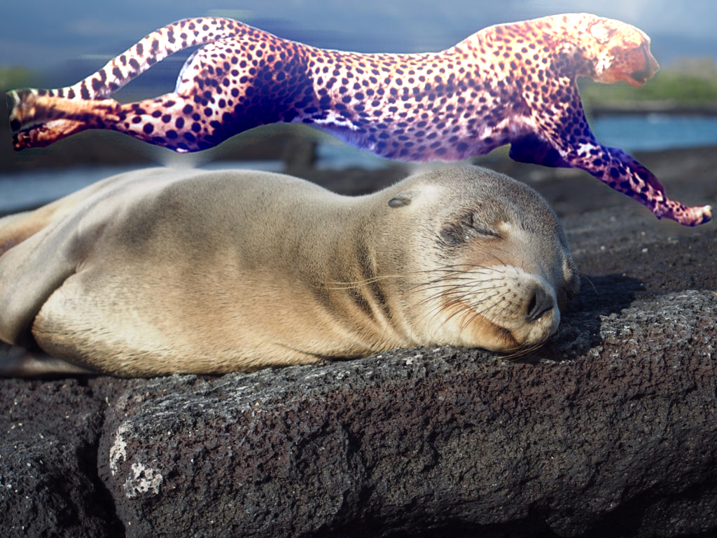
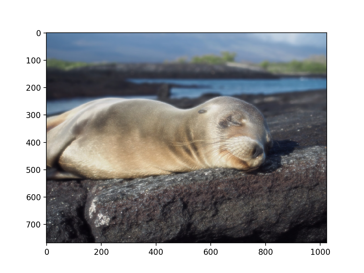
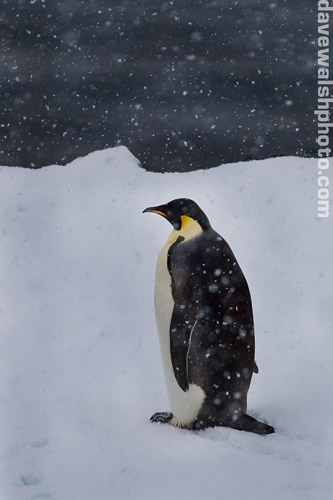
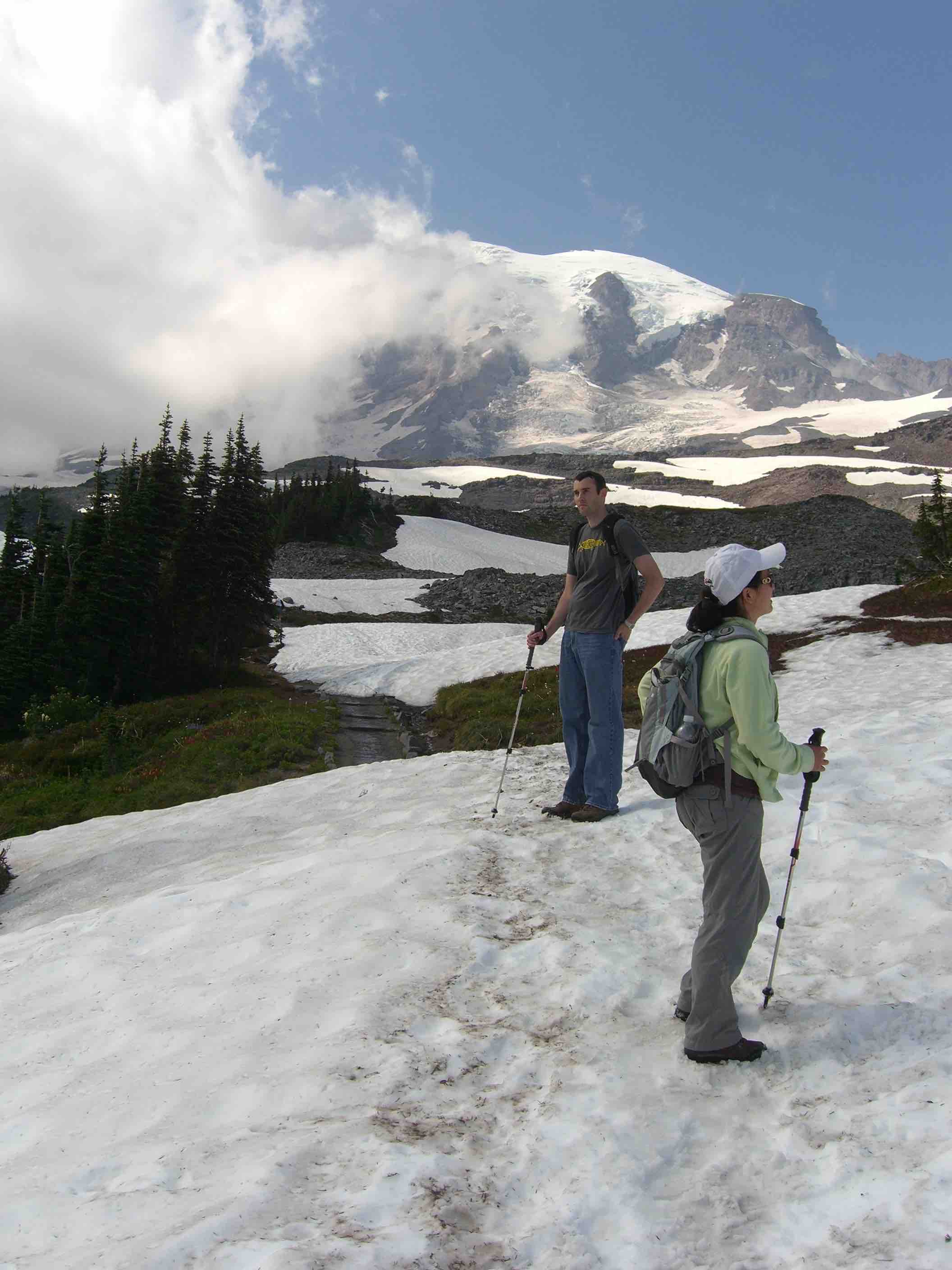
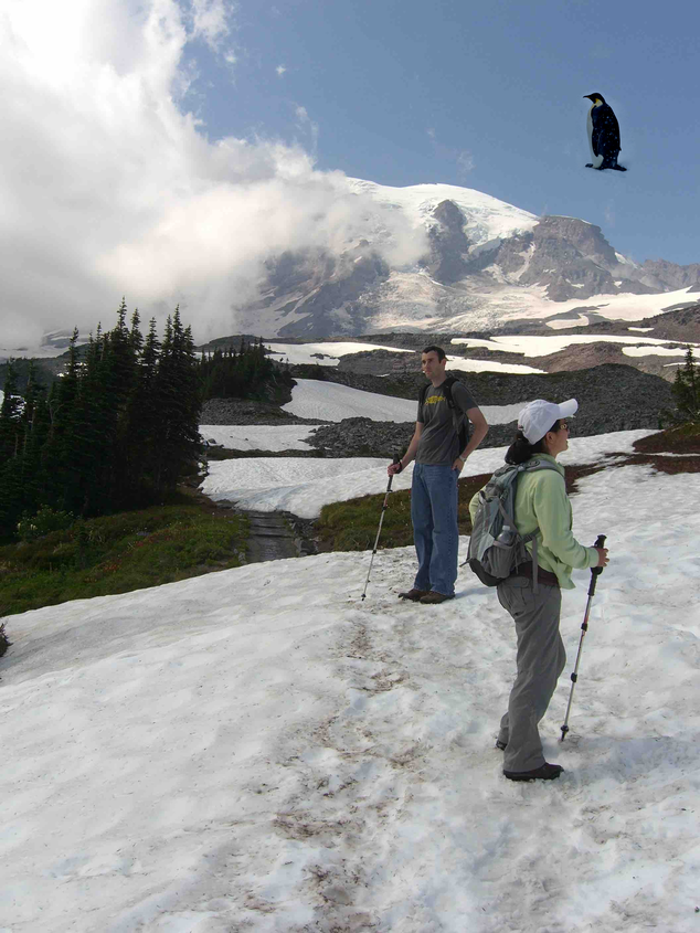
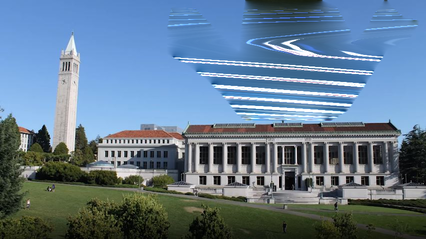
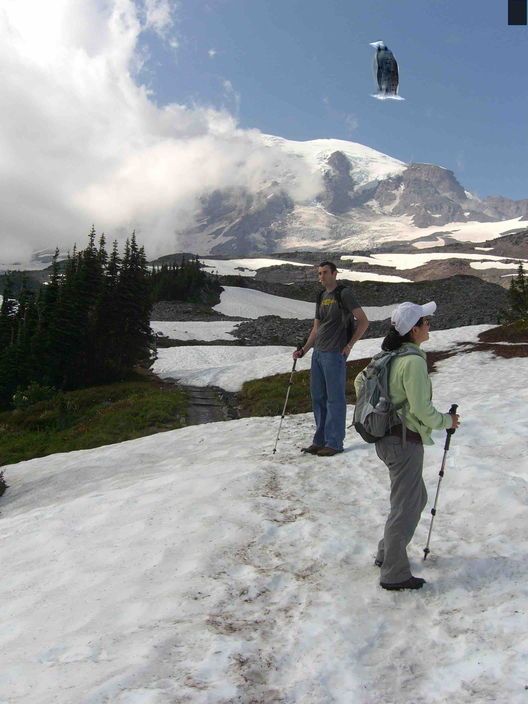
For this part, I combined two images in a way that would mix the features from one and apply them to the other image. I did this by applying a low pass filter two one image, meaning that only the low frequencies of one of the images would show. I then applied a high pass filter with a different cutoff to the other image, meaning that there would be no frequencies present in between the frequencies. By combining these images, I could then get one composite image that differs in appearance when viewed close up (and seeing the frequencies from the high pass filter) than when viewed from far away, where you can only see the low frequency images.
1.4 Multiresolution Blending:
In this part, I blended two images by feathering each element of the gaussian stacks of the two images. This technique was used to minimize the starkness of the seam between the two images, and therefore make the translation more seamless.
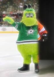
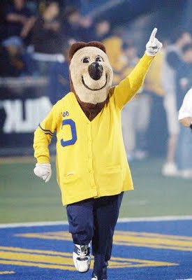
- This blends the right arm and leg of Gritty, the Philadelphia Flyers mascot with that of Victor E. Green, the Dallas Stars mascot
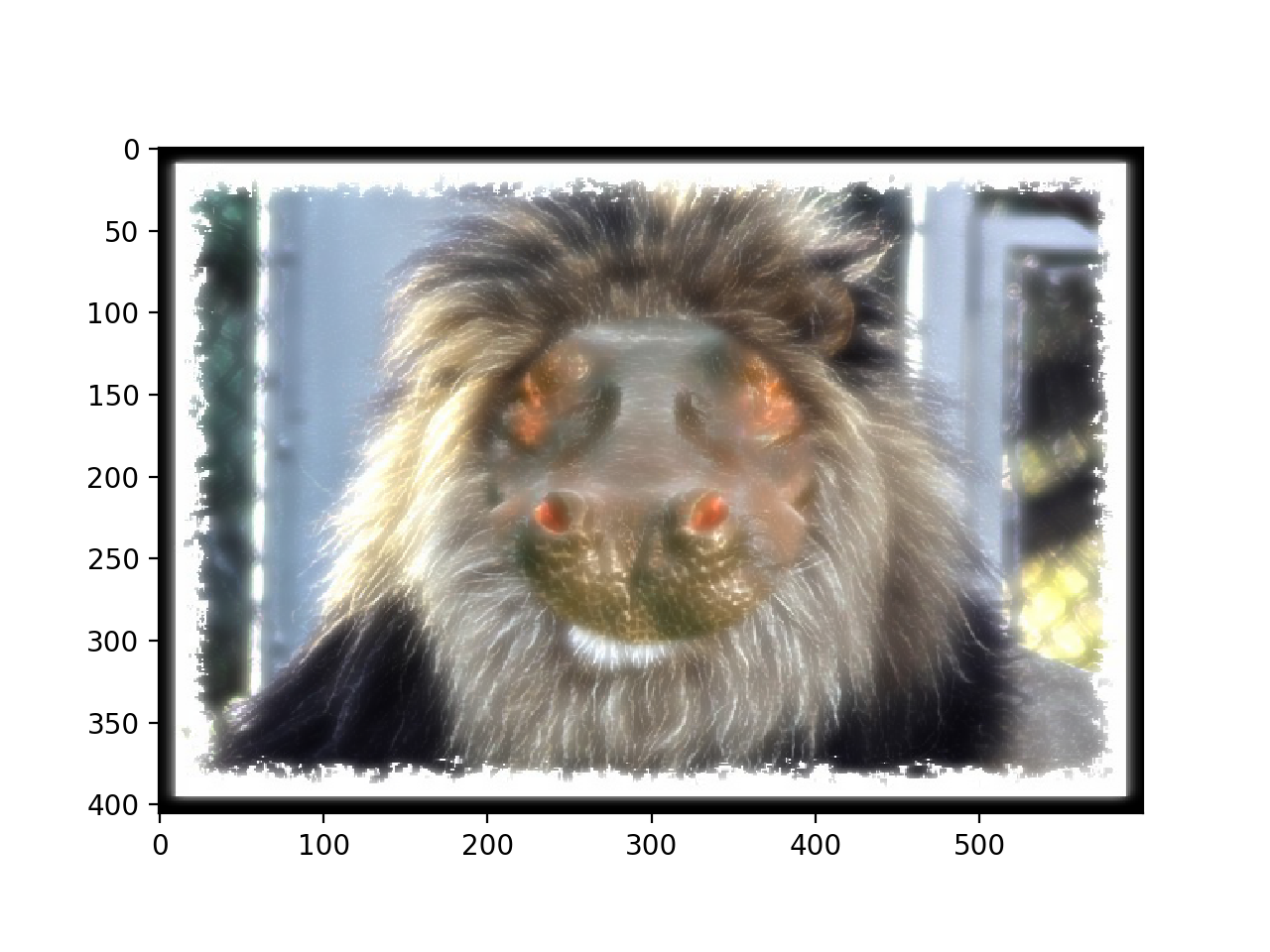
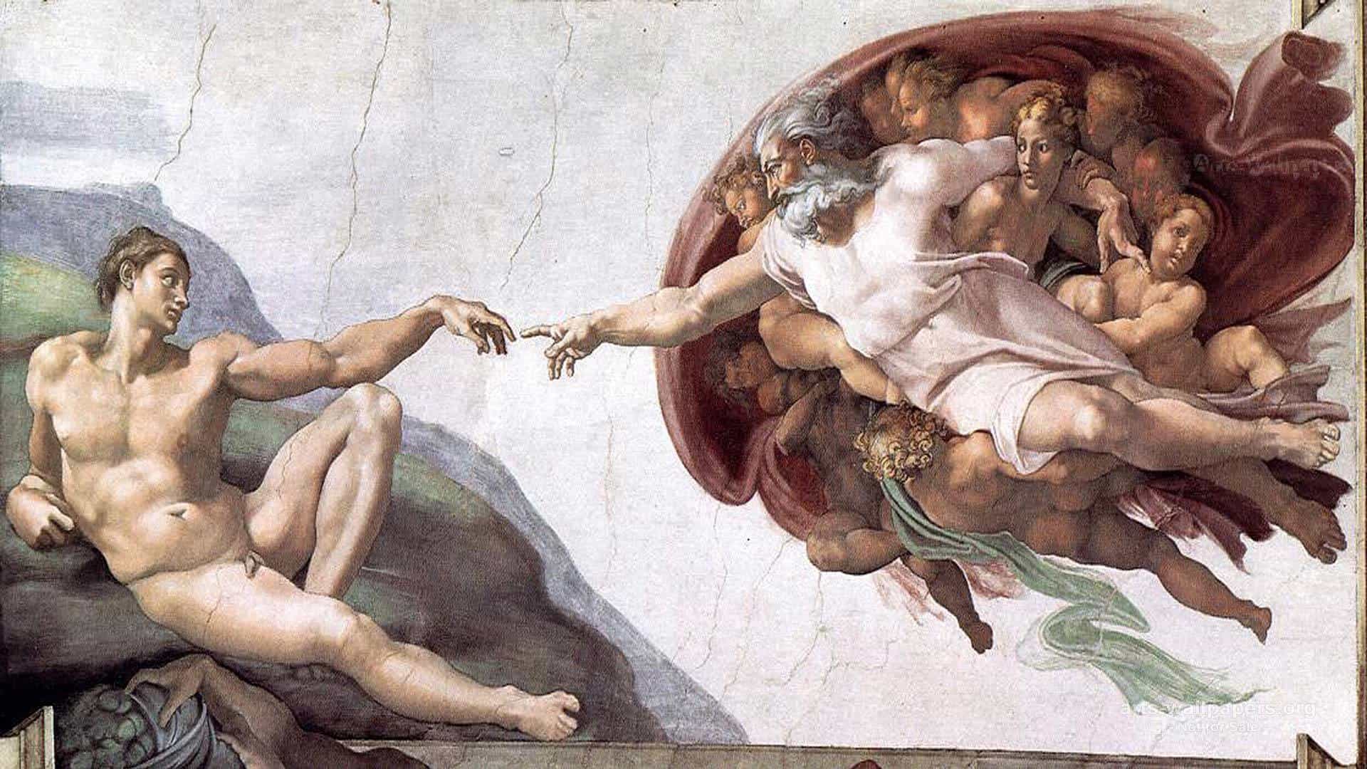
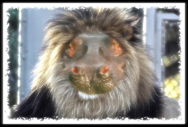
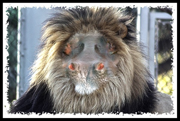
- This was putting the face of a hippo inside the mane of a lion
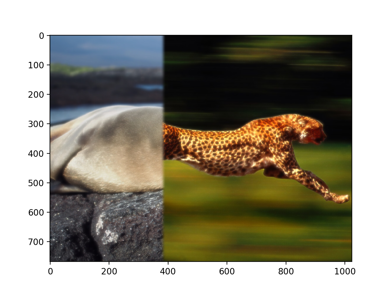
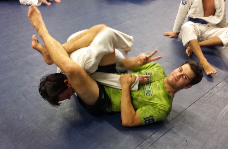
- This was a failure, since there was not a nice common seam between the images, so they didn't align well.
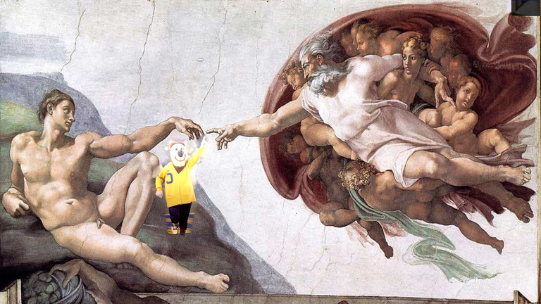
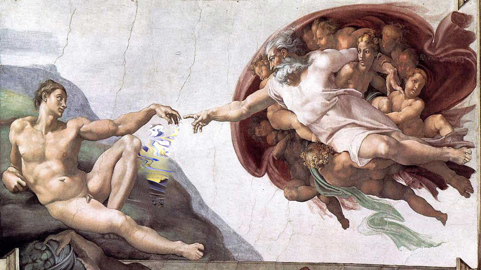
Poisson blending
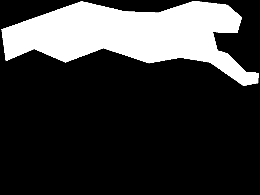
For the second half of the project, I implemented Poisson blending as a way to combine two images. To do this, I had to try and minimize the difference between the images on the borders, ensuring that when you place what you are adding in to the other image, there is a minimal border between images. I can do this by solving the least squares problem:

To solve this, I have to find a vector v, that when it is inside the image matches the original superimposed image, but when on the border matches the border as close as possible. I did this by populating a sparse matrix with the locations of each pixel.
2.1 Toy problem
For this part, I implemented a special case of poisson blending, where there was only 1 image, and I wanted to recreate the image from just one pixel value and the differences between the pixel values.
| Source |
Reconstructed |
 |
 |