Warmup
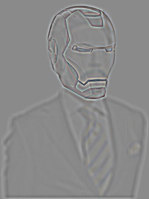
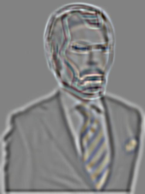
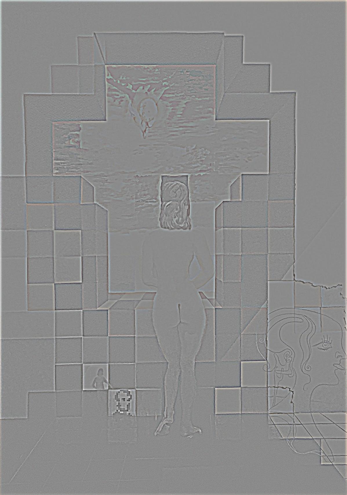
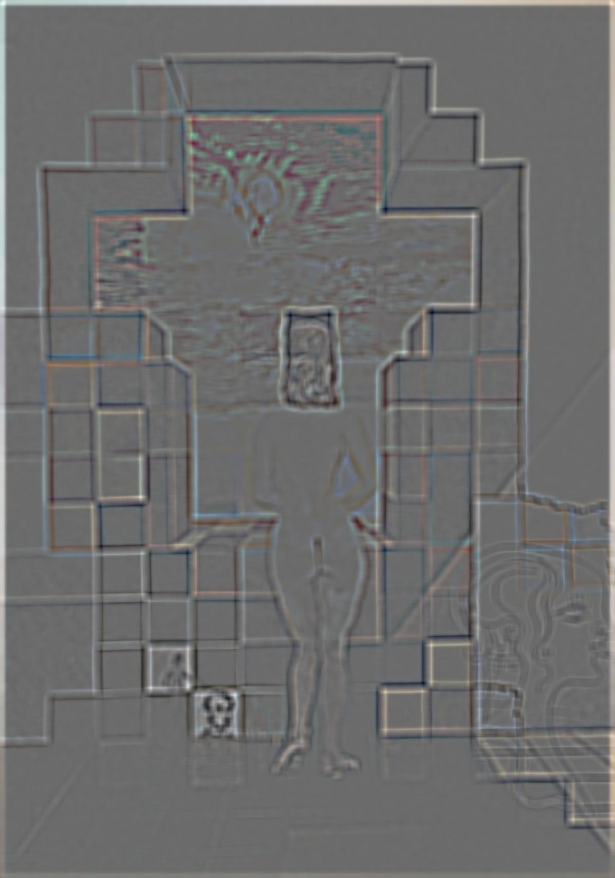
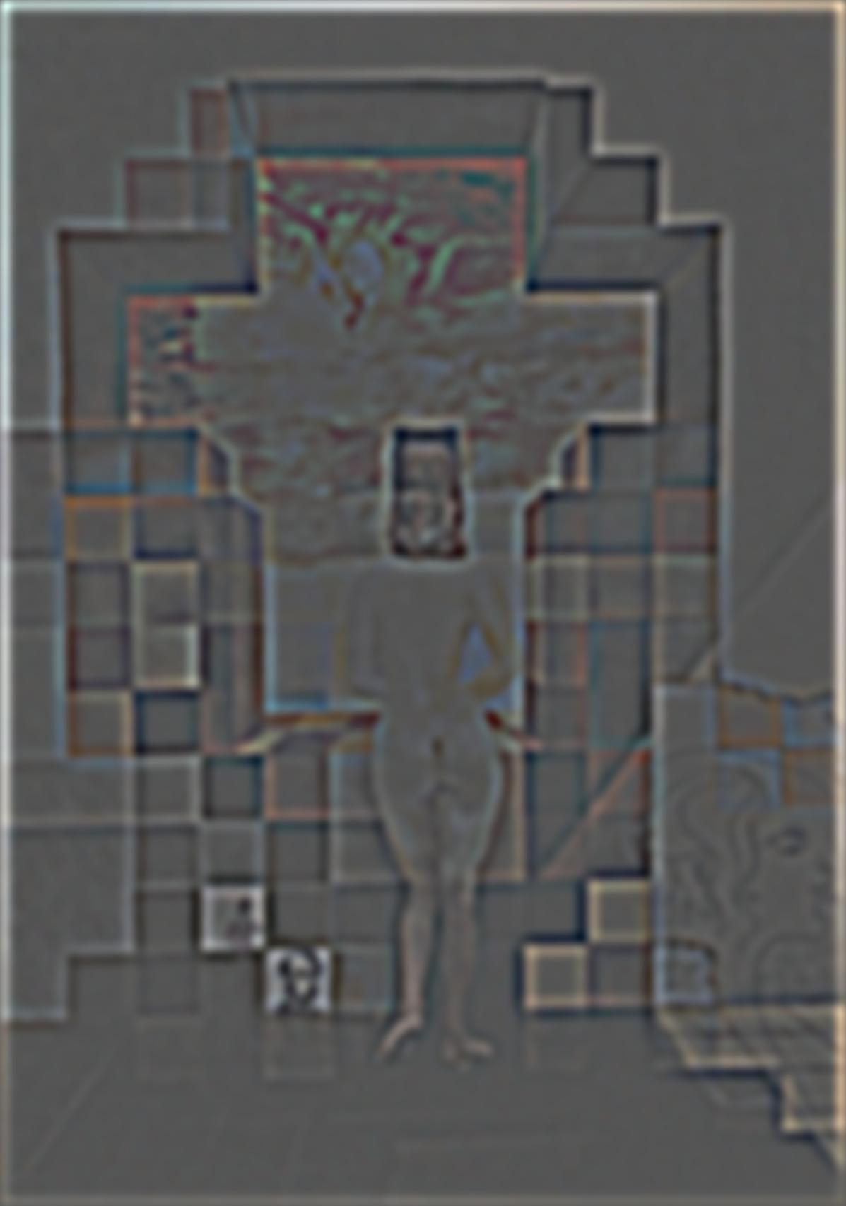
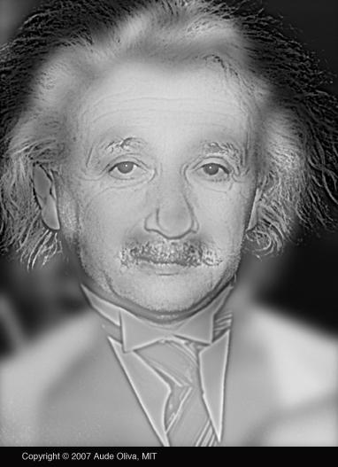
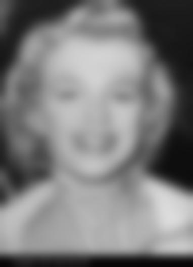
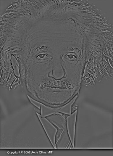
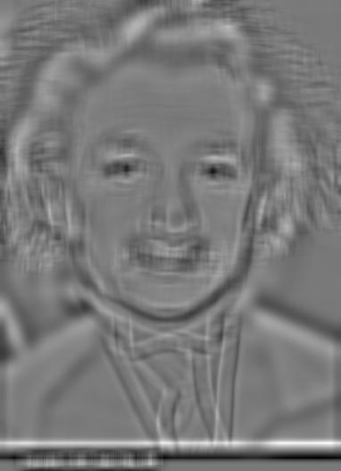
To create a sharpening effect, we want to compute the high pass filter of an image. To do so, we can put a picture through a Gaussian filter to obtain a blurred photo. To get a Gaussian filter we must calculate a kernel and then apply a 2D convolution to the image to perform a Gaussian blur. Then we can subtract the blurred image from the original image to get the details, or the high pass filter. Next we add the details to the original image, creating a sharpened look.

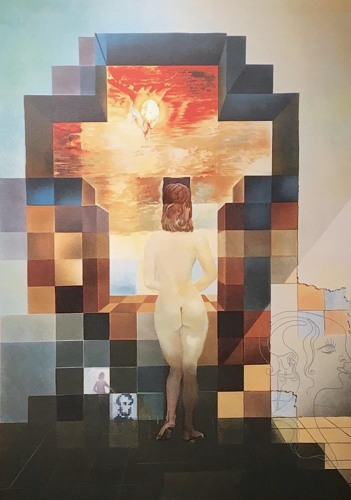
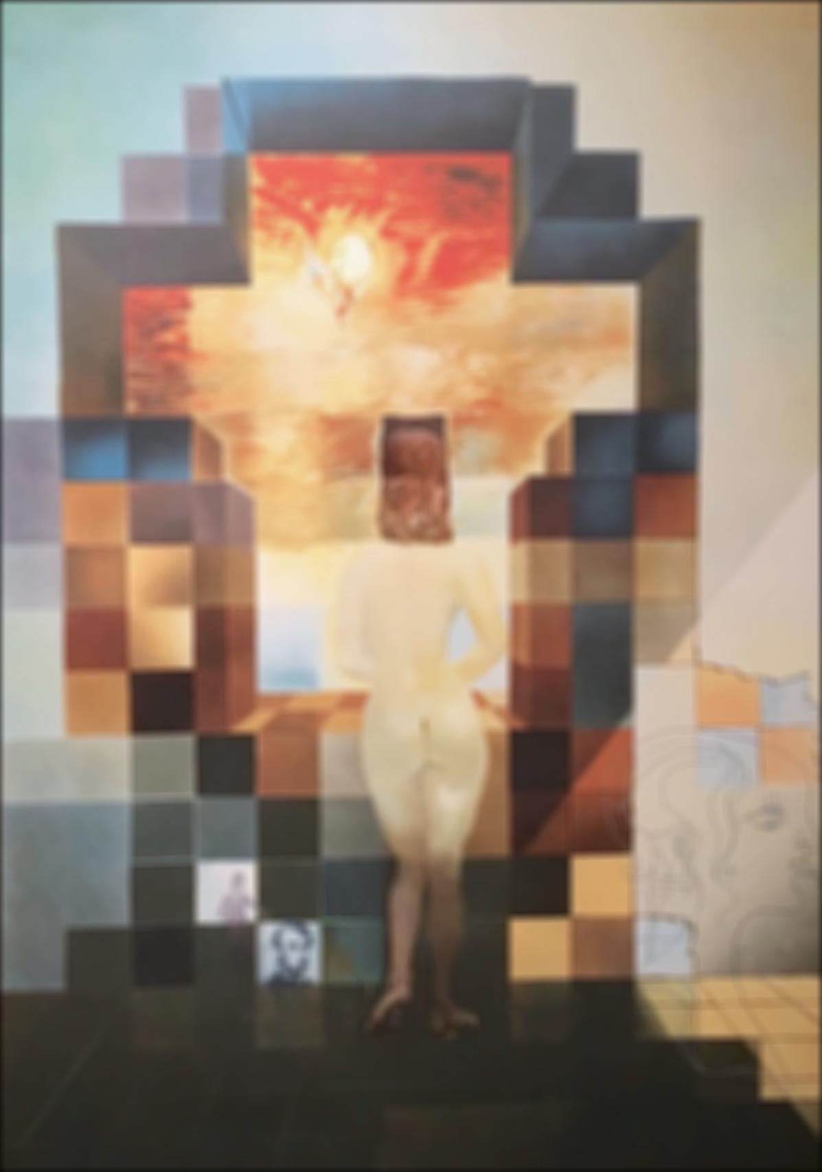
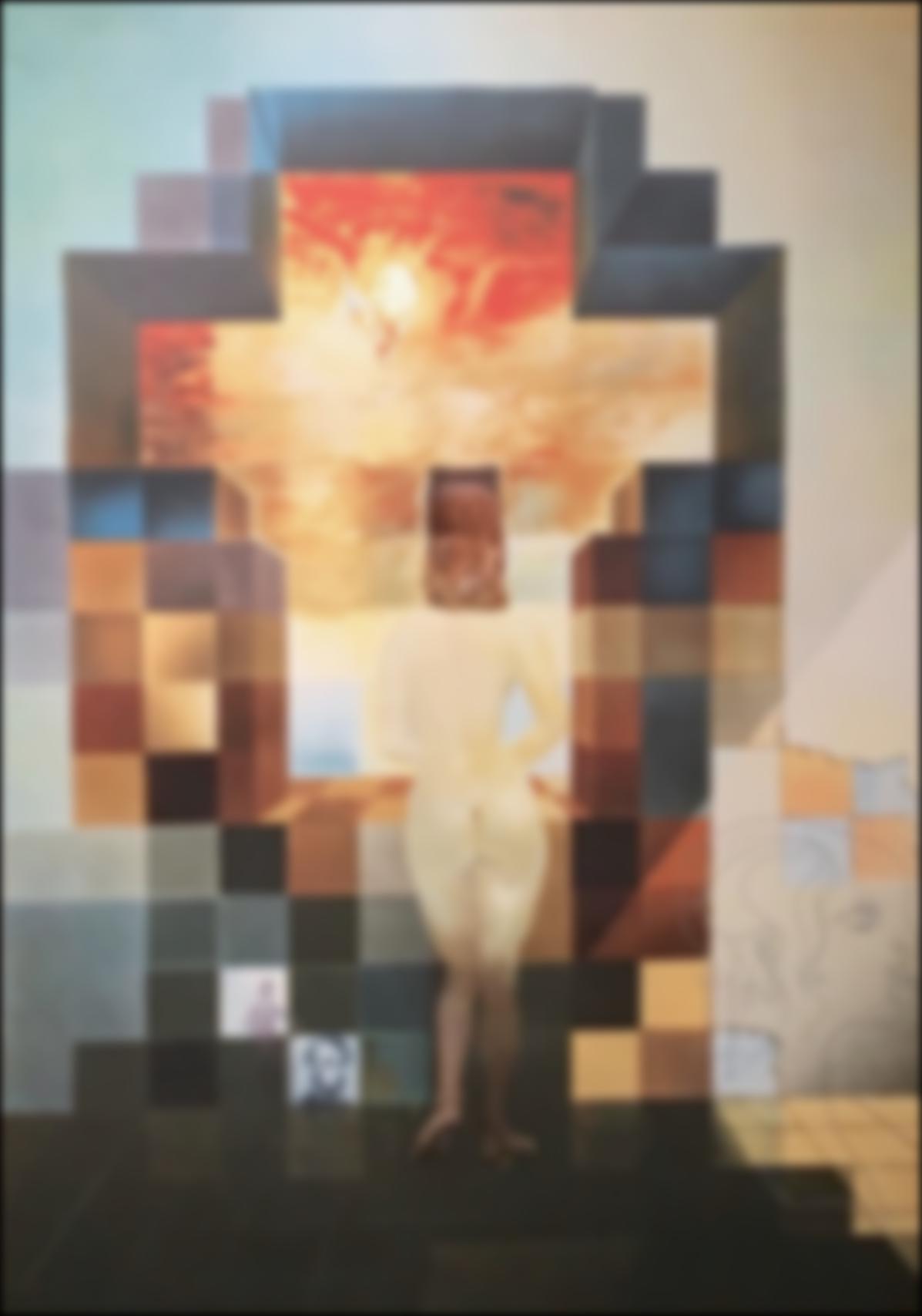
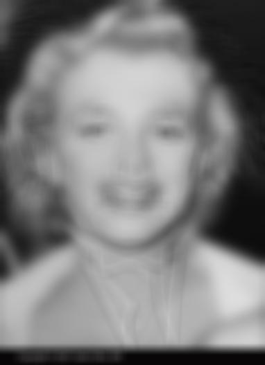
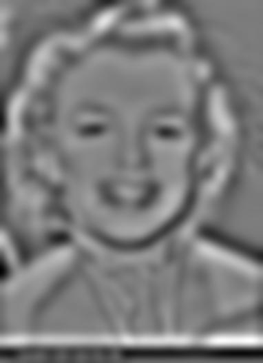
Original

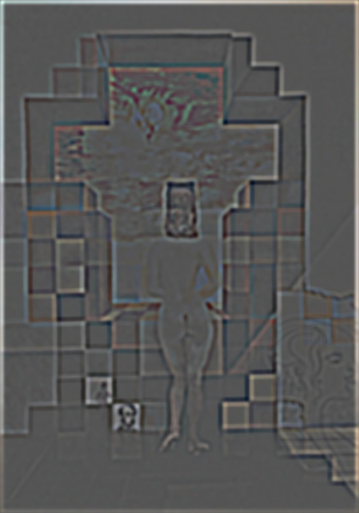
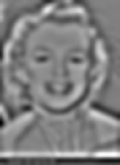
"Sharpened"