The purpose of this project is to explore different methods of blending images together.
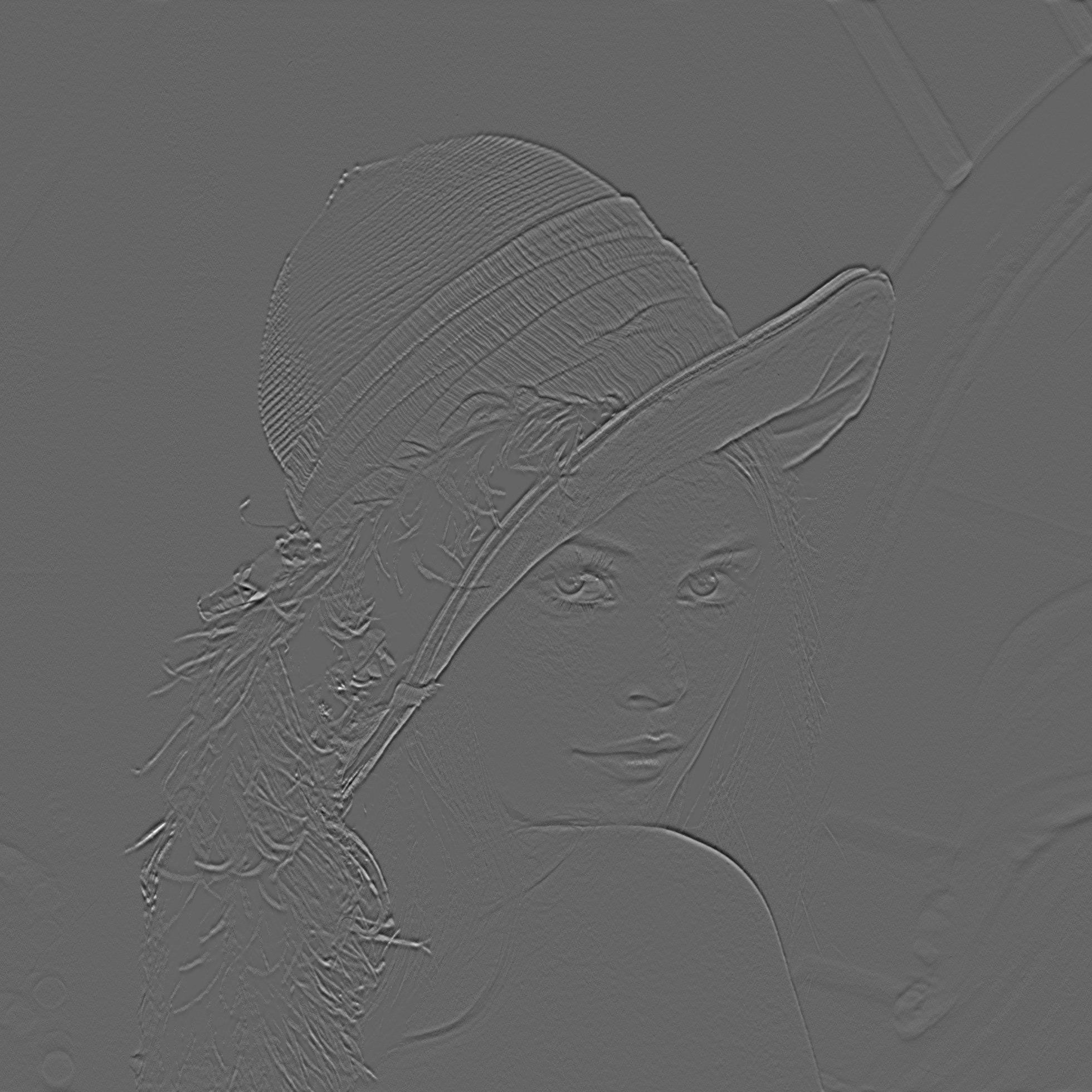
I applied a Laplacian filter on the original image using a kernel of size 21 and sigma 5 in order to obtain the high frequency details of the image. Next I multiplied the Laplacian image with a chosen alpha value and added the result to the original image. This yielded a sharpened version of the image.


Here is one failure case. It is very difficult to see Michelle Obama's face.


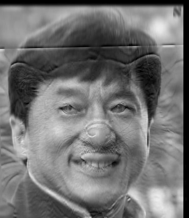
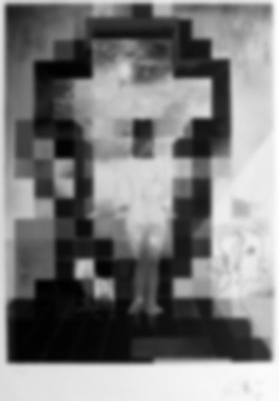
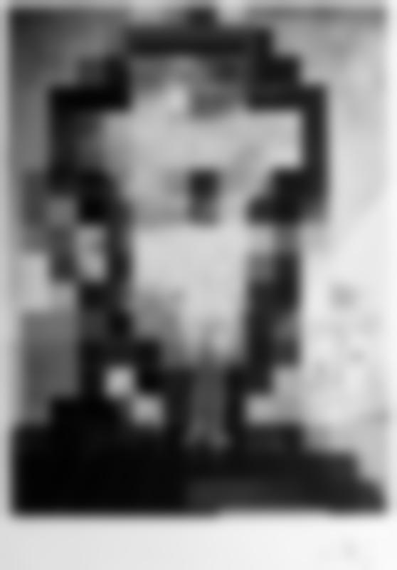
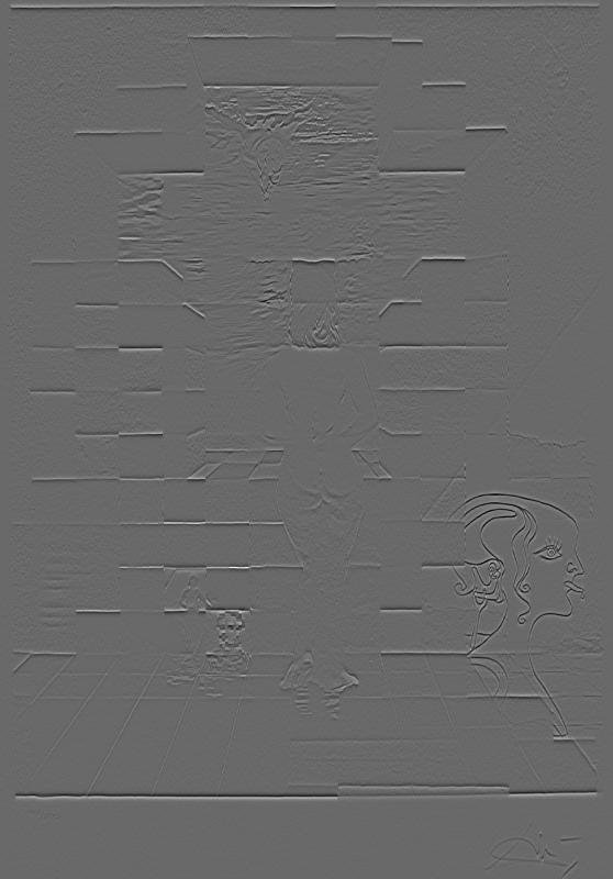
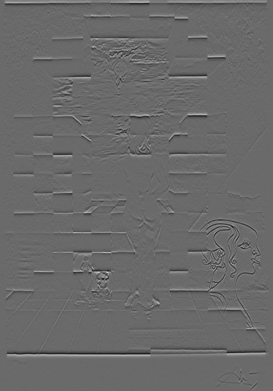
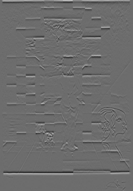
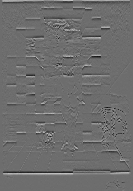
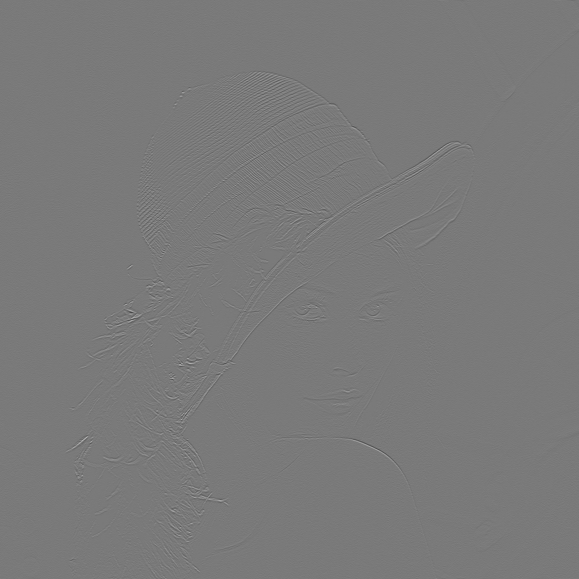
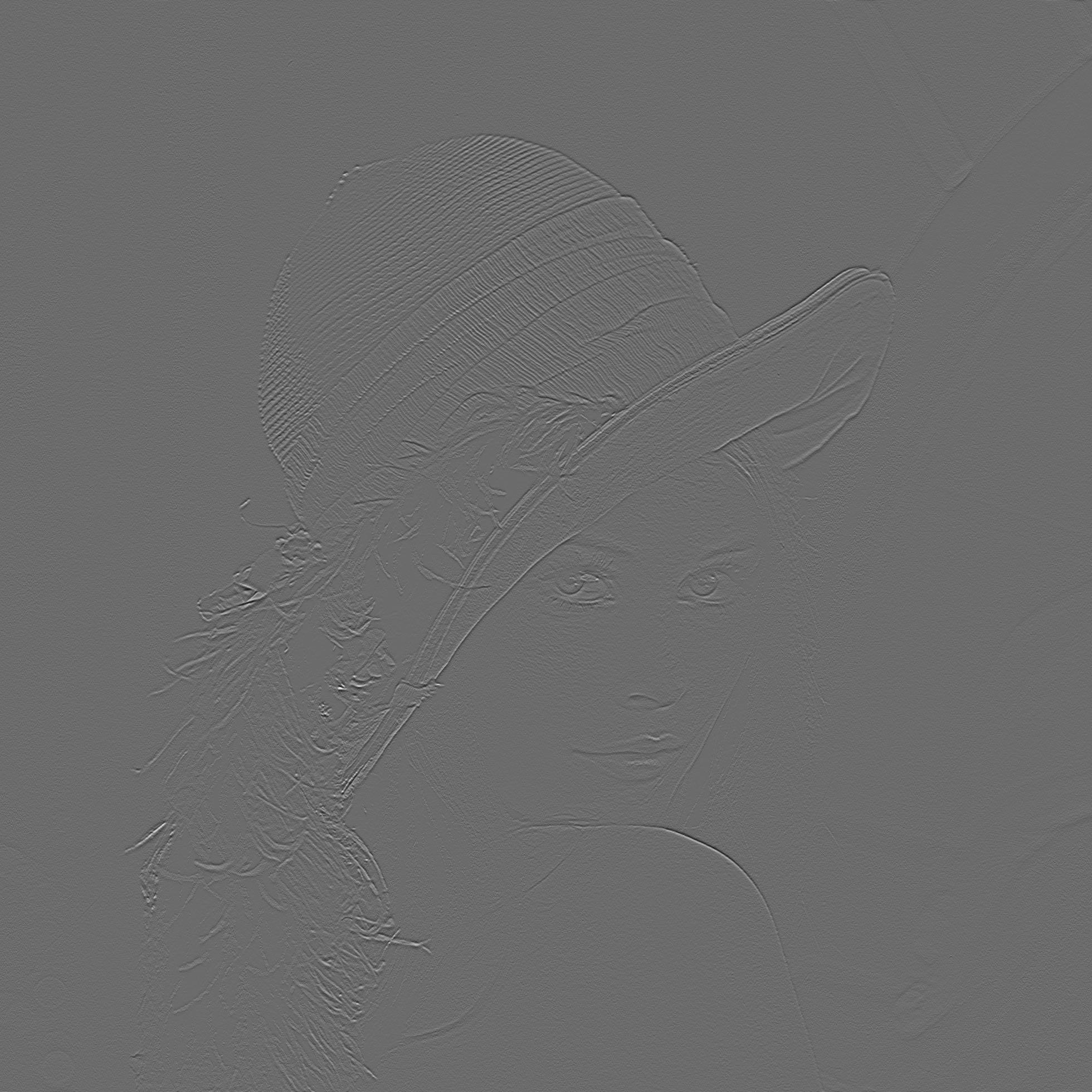
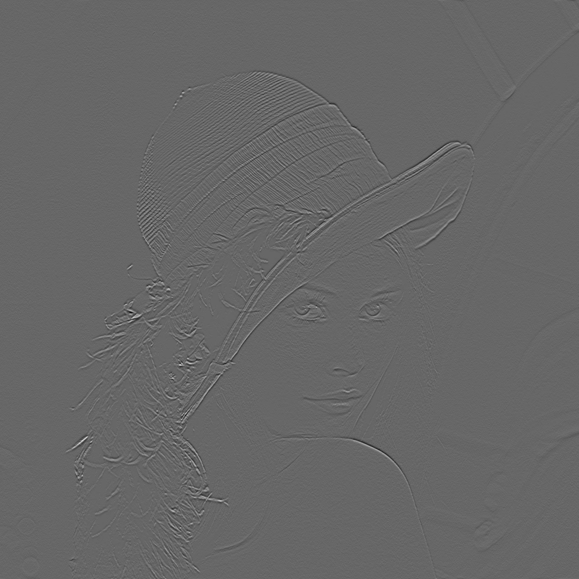
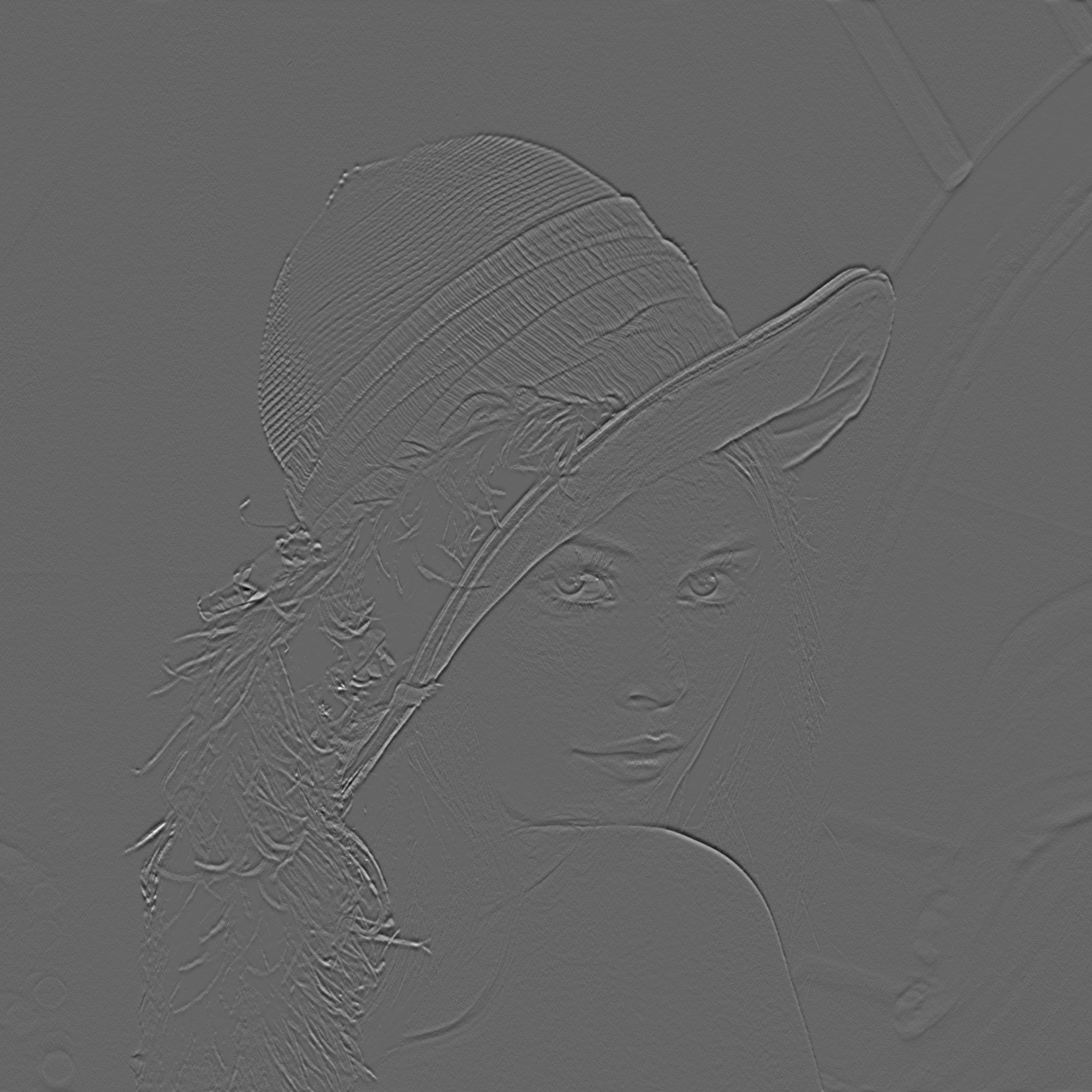
To create Gaussian stacks, I applied the Gaussian filter on the image repeatedly while increasing the sigma value by a factor of two. To create the Laplacian stacks, I applied the Gaussian filter on the image and subtracted it from the previous image while increasing the sigma value by a factor of two. For both Gaussian and Laplacian stacks I started with a sigma value of 1. The pictures below show stacks with sigma equal to 1, 2, 4, 8, 16, and 32. We see that as we increase the sigma for the Gaussian stack, the Lincoln Dali image gts very blurry. Interestingly, as we increase the sigma for the Laplacian stack, it gets easier to see the Lincoln Dali image since we are getting more of the high frequency details.


Multiresolution blending uses splines to help blend two images together without there being a sharp seam between the two combined images. Given two images, we create Laplacian stacks of them (LA, LB). Next we create a mask and create a Gaussian stack for it (GM). For each level of the stacks, we assemble a combined stack by doing the following: LA_i * GM_i + (1 - GM_i) * LB_i.


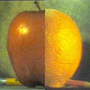
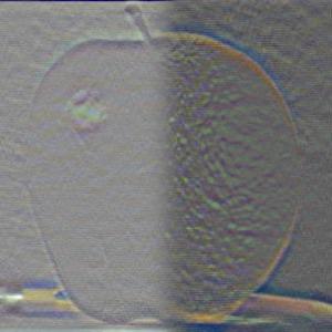
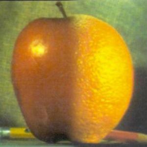
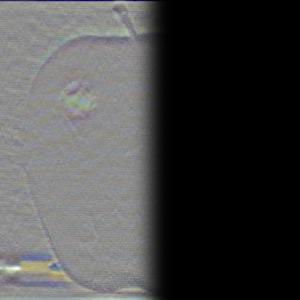
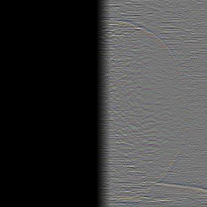
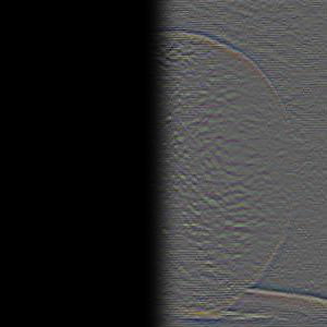
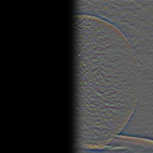
Here are the Laplacian stacks for the apple and orange.

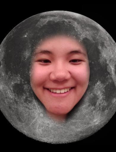
A blend with an irregular mask.
Given a pixel and the gradient of the original toy image, we reconstruct the image using a system of equations. We create a sparse matrix A with dimensions ( * height * width + 1, height * width). Note that the number of rows we have in A represents the number of equations we are trying to solve for. The first half of matrix A corresponds with the x-gradient while the second half corresponds with the y-gradient. The last row of matrix A helps make sure that the top left corners of the two images are the same color. We multiply this matrix A to vector x which represents all the unknowns we are solving for - the mapping between a given pixel to the reconstructed image. So we now have Ax = b. The vector b with dimensino (2 * height * width + 1, 1) represents the result of the gradient equations in matrix b.

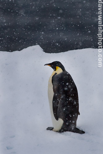
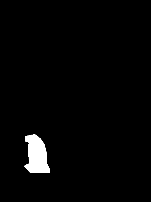
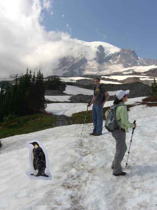
In Poisson Blending we look at the gradient of an image and attempt to find values for the target image that maximally preserve the gradient of the source image without changing any of the background image. For each pixel i outside the masked region, the output image pixel is the same pixel as the target image. For each pixel i inside the masked region, the output image pixel depends on its left, right, above, and below neighbors. We construct a sparse matrix A (# target rows * # target cols, # target rows * # target cols) and a vector b (# target rows * # target cols, 3 RGB). We can plug this into a least squares solver to obtain the solution that encodes the correct pixel value from source to target image.