CS194-26 Project 3

Michael Weymouth (cs194-26-adc)

Description

This project explored various methods of blending images with frequencies and gradients. We started with an examination of various methods of overlaying and blending methods through Gaussian and Laplacian frequency analysis, while also exploring the frequency domain effects of such methods. Then, we took a detour into gradient domain processing using least squares, allowing us to blend images while minimizing visible seams.

Part 1.1: Warmup

In this part of the project, we first perform a Gaussian filtering of the image, then we subtract this blurred portion from the original image to get a high-pass version of the image. Finally, we add back this high-pass version of the image scaled by a constant factor a to obtain the sharpened image. Below, you can see the results of applying this procedure to the famous Lenna image.

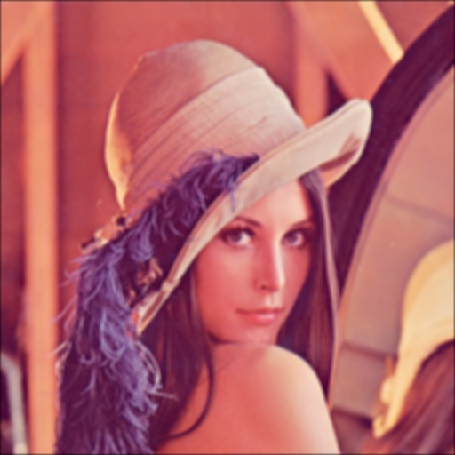
Before sharpening

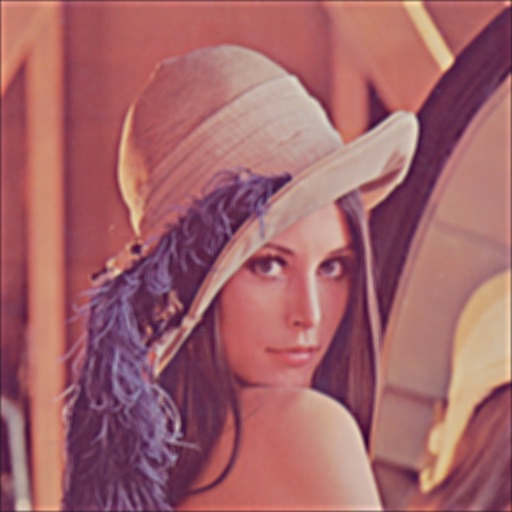
After sharpening (filter size: 15, a: 0.5, sigma: 10)

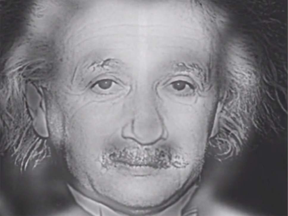
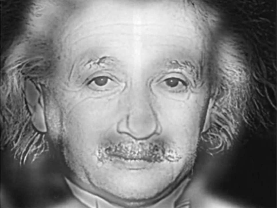
Part 1.2: Hybrid Images

This part was performed by first aligning the images with the given code, then running one image through a high-pass filter and the other through a low-pass filter. The two images were then overlaid to form the hybrid images you see below!

Batman and Bruce Wayne can’t be seen at the same time, interesting…

Batman: (filter size: 21, sigma: 10)

Bruce Wayne: (filter size: 21, sigma: 0.8)

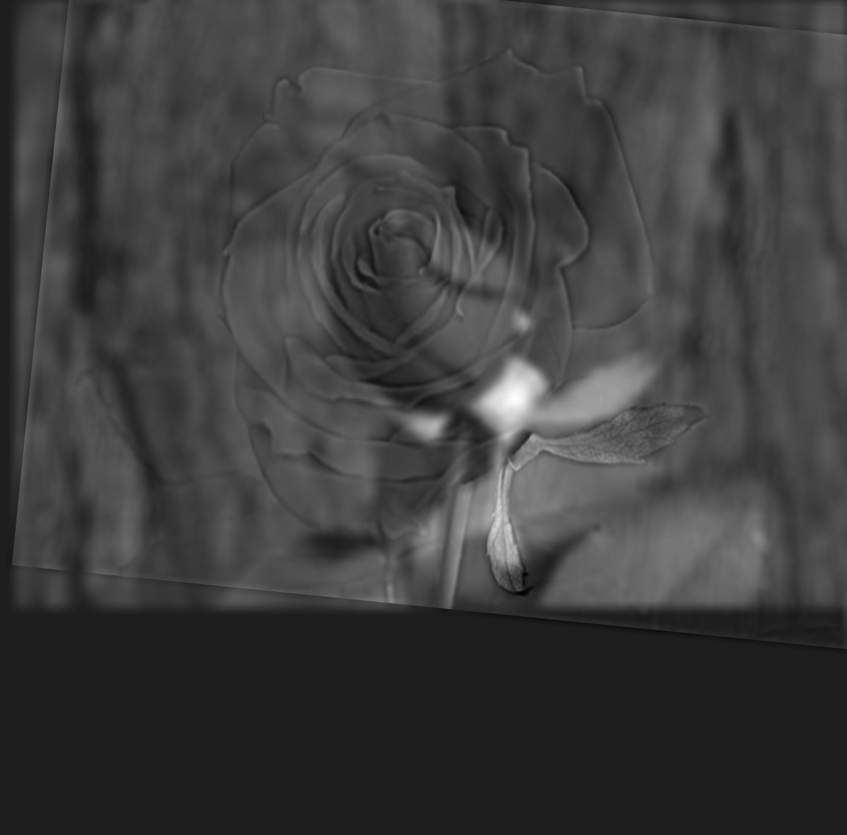
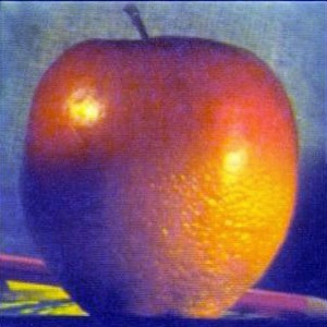
A rose (sort of) blooms, right before your eyes!

(This is a failure case: the background low-pass rose is always visible, even up close.)

Closed: (filter size: 21, sigma: 20)

Bloomed: (filter size: 21, sigma: 10)

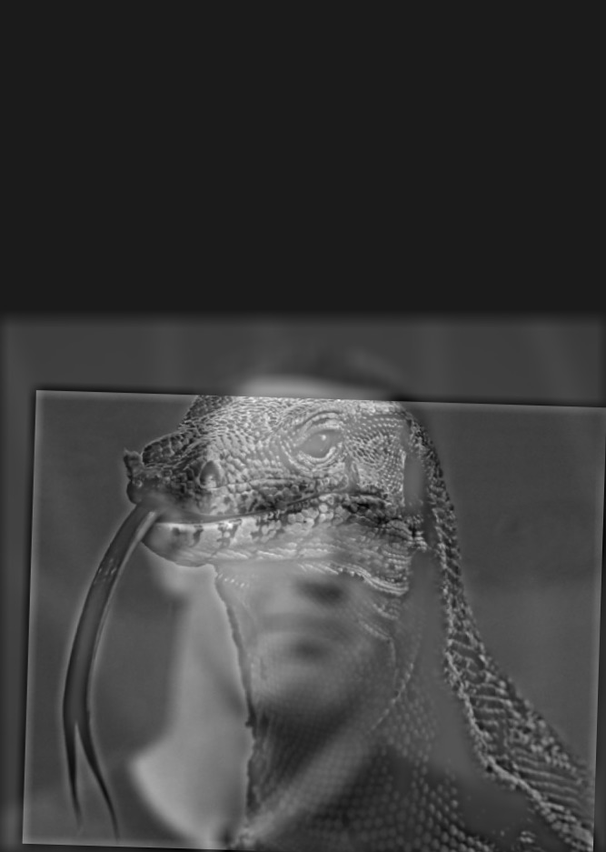
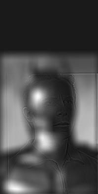
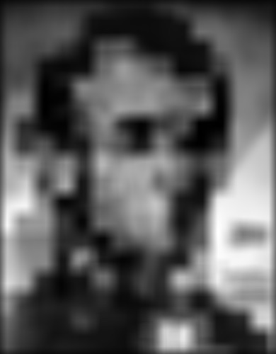
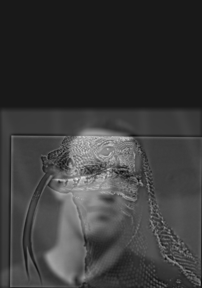
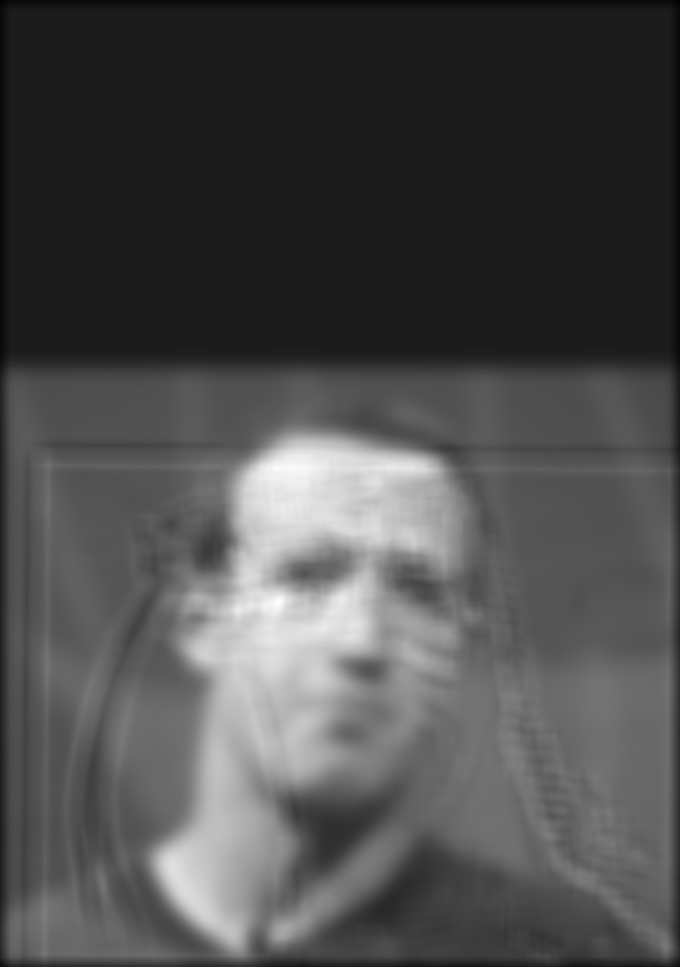
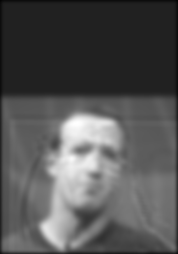
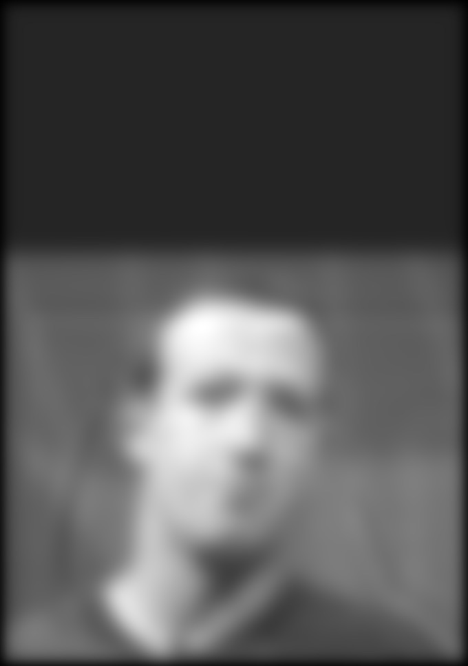
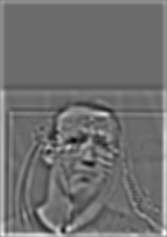
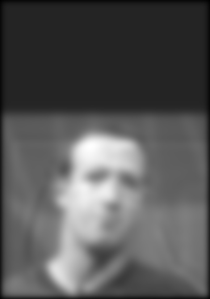
Up close, Mark Zuckerberg reveals his true form…

Mark Zuckerberg: (filter size: 21, sigma: 20)

Lizard: (filter size: 21, sigma: 10)

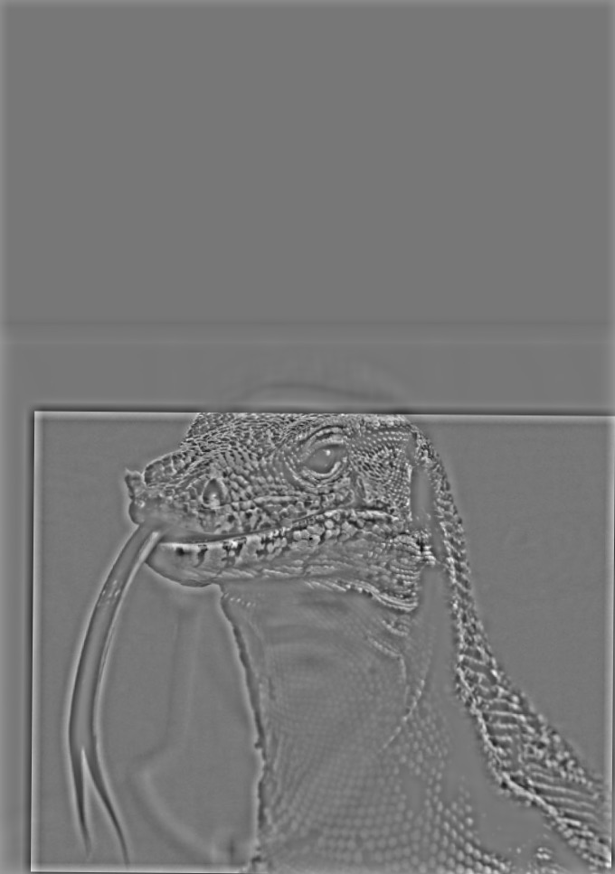
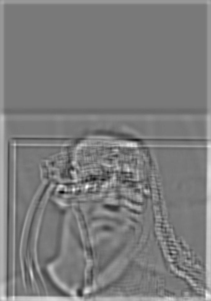
We can analyze this image further, by taking the Fourier Transform at several points in the combination process.

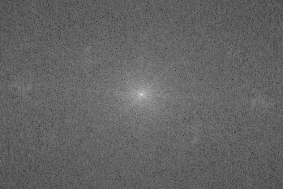
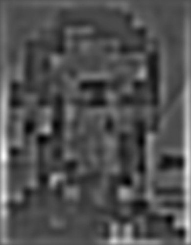
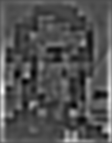
The Fourier Transform of Mark Zuckerberg.

The Fourier Transform of a lizard.

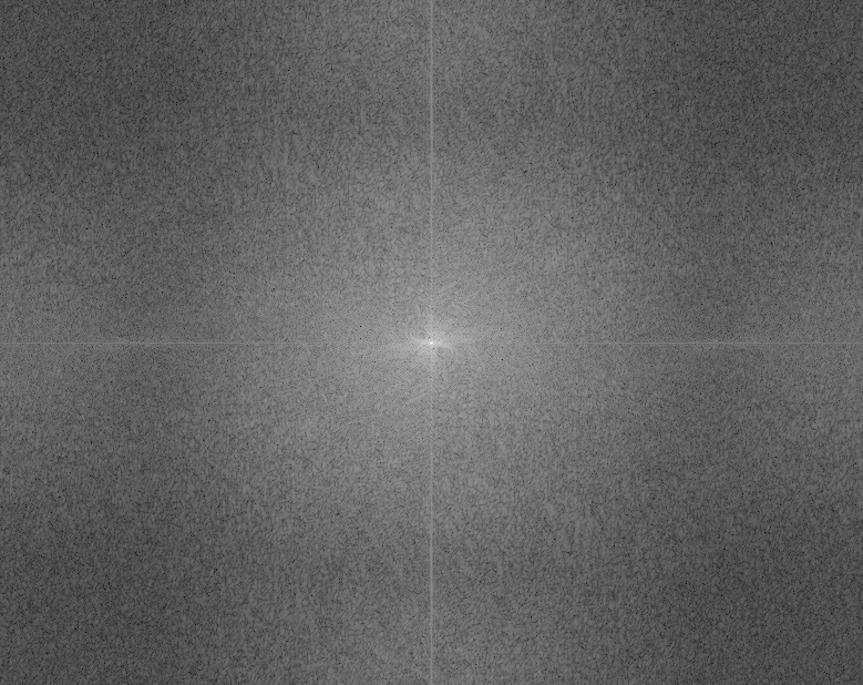
The low frequency Zuckerberg image FT after filtering.

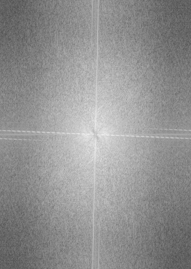
The high frequency lizard image FT after filtering.

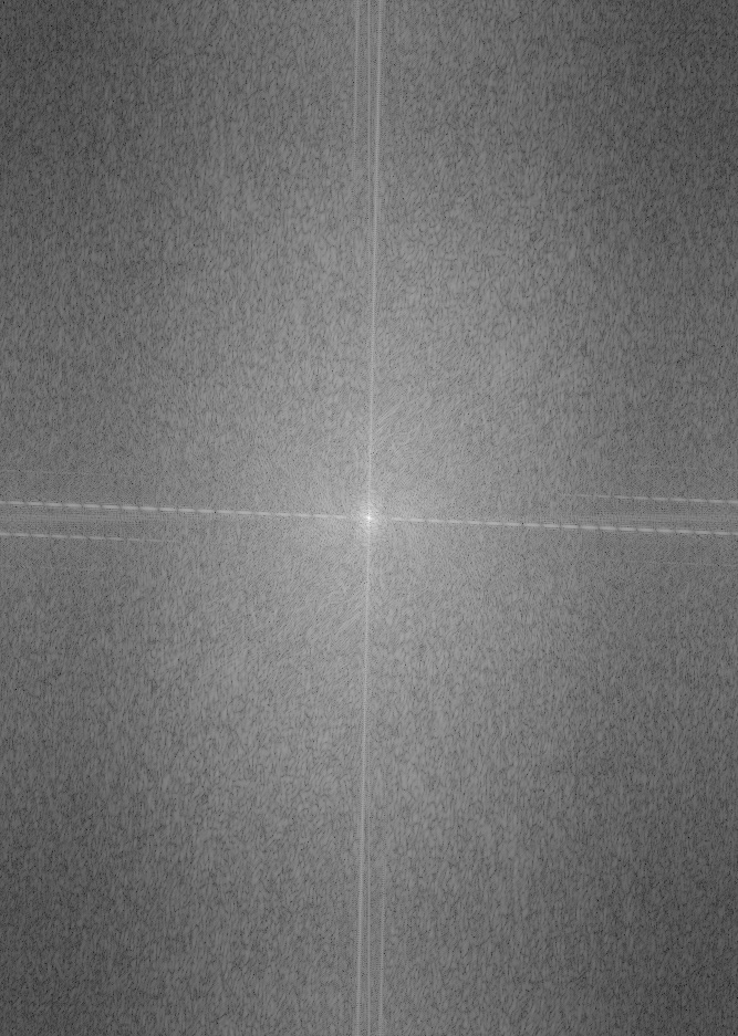
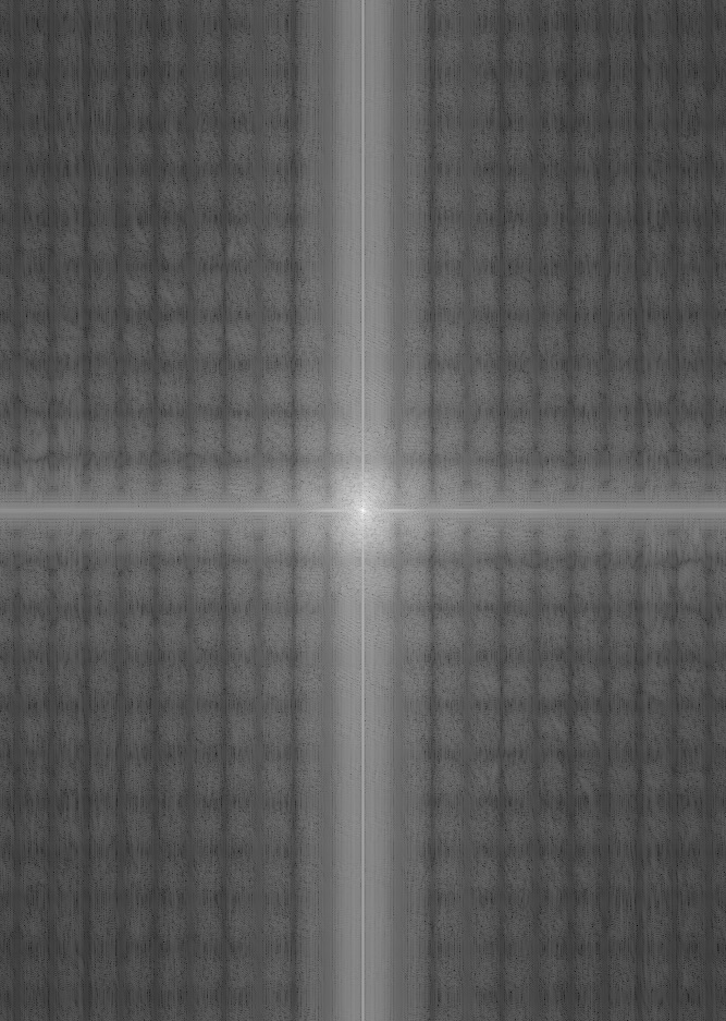
The Fourier Transform of the hybrid image.

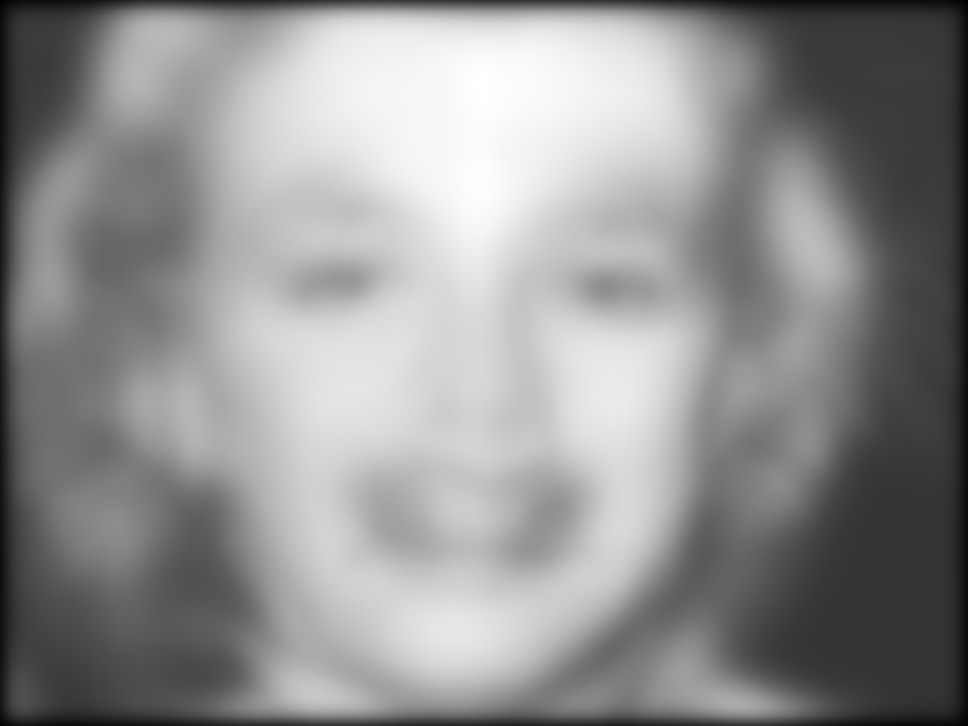
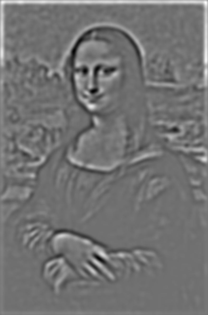
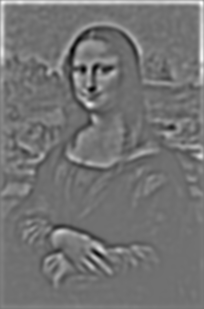
Part 1.3: Gaussian and Laplacian Stacks

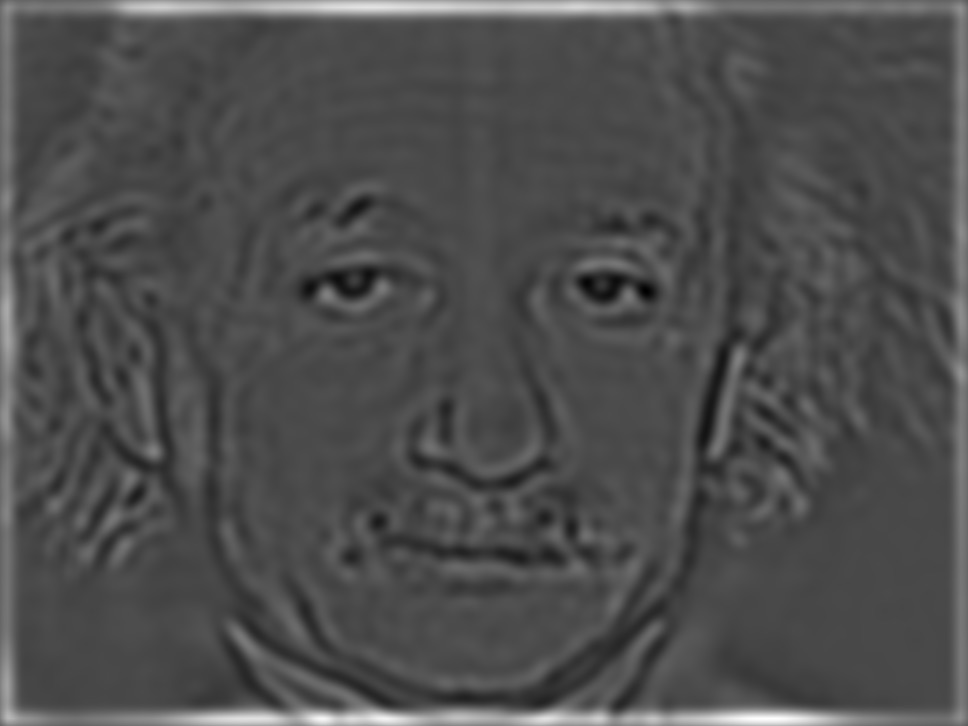
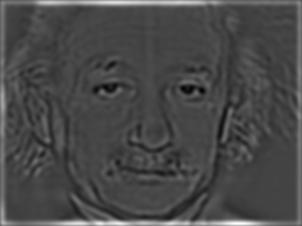
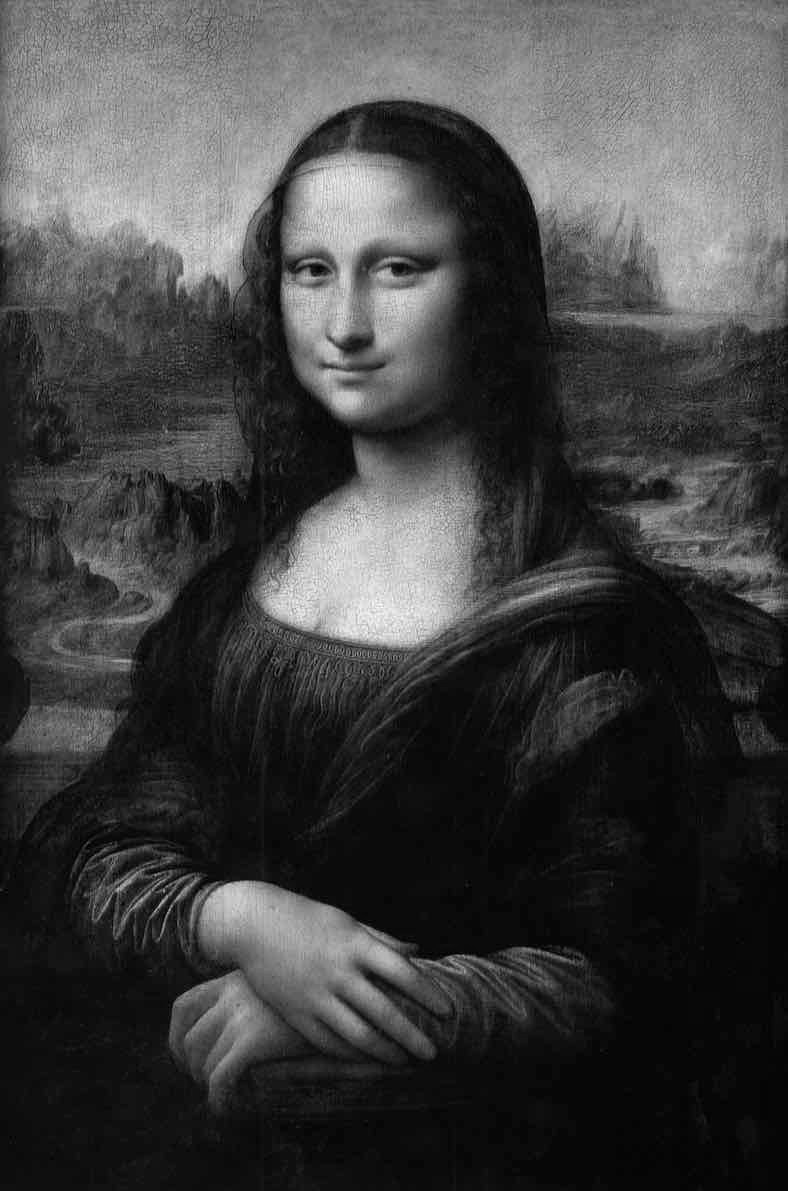
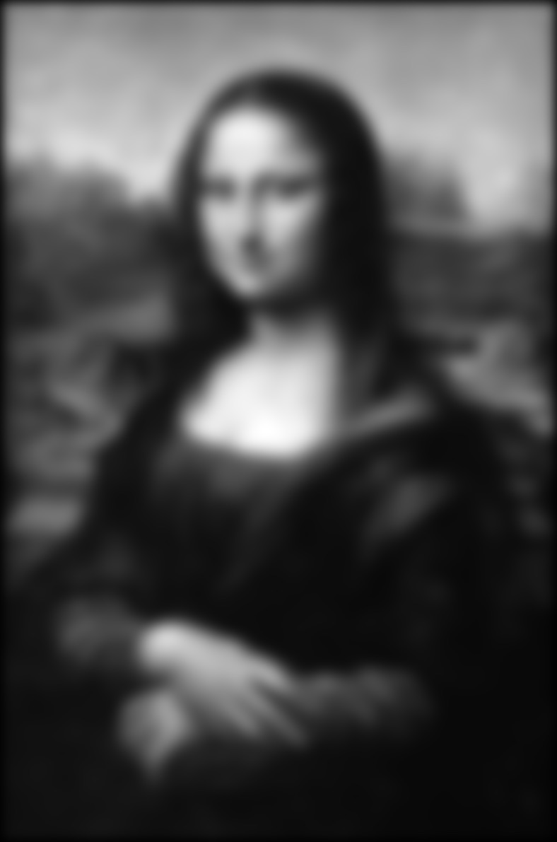
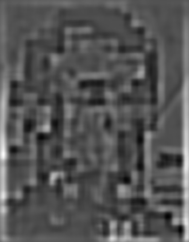
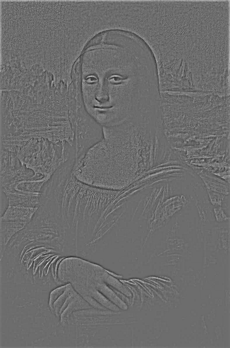
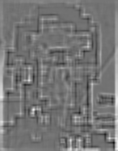
The Gaussian Stack was implemented by taking an input image and repeatedly applying a Gaussian filter to the image, saving it in an array at each step. The Laplacian Stack was implemented by generating a Gaussian Stack of size N, then calculating each entry i by subtracting the (i + 1) entry of the Gaussian Stack from the i entry. Lastly, the Gaussian entry at N is appended to the Laplacian stack, and the stack is returned.

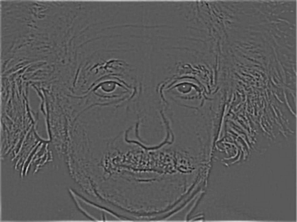
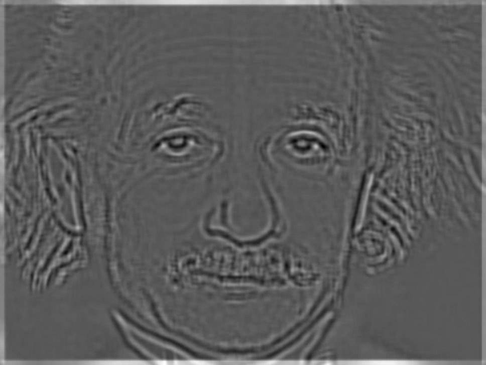
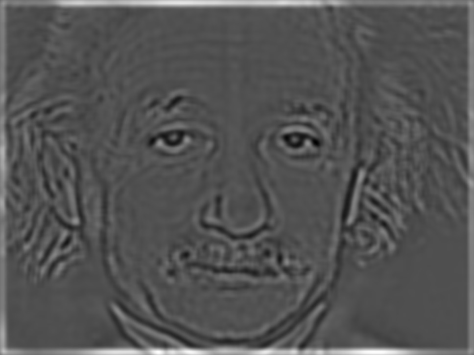
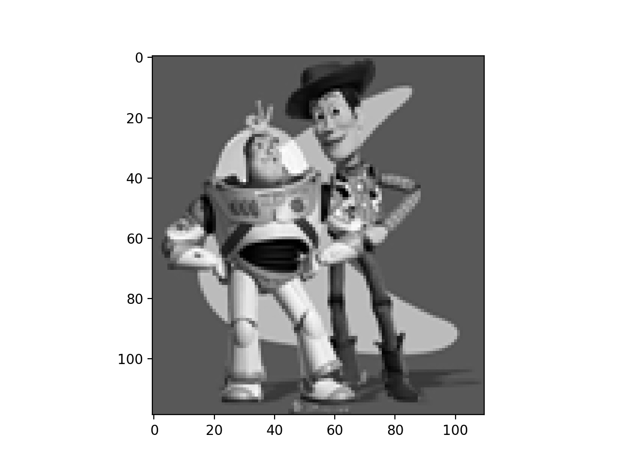
For all of the example images below, a filter size of 21 and sigma of 15 were used.

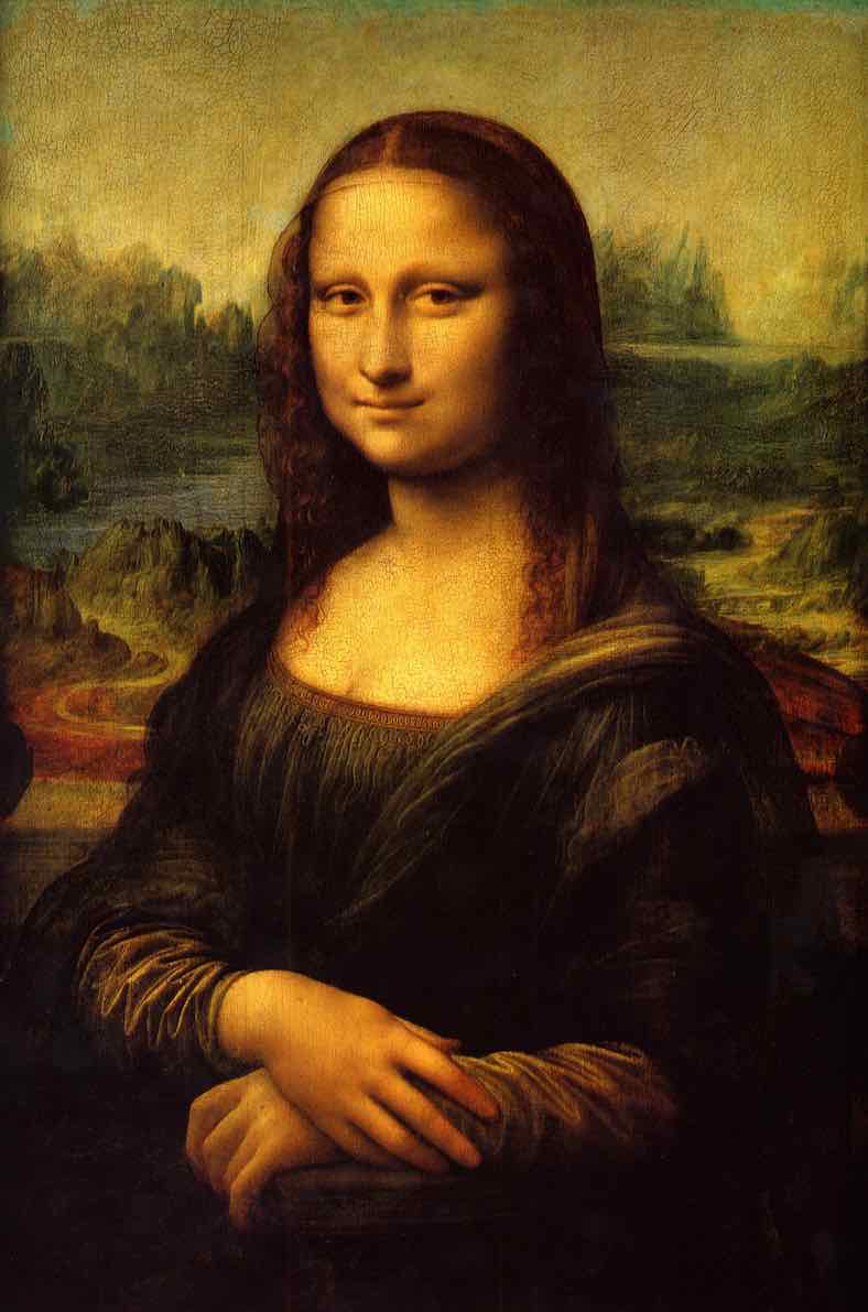
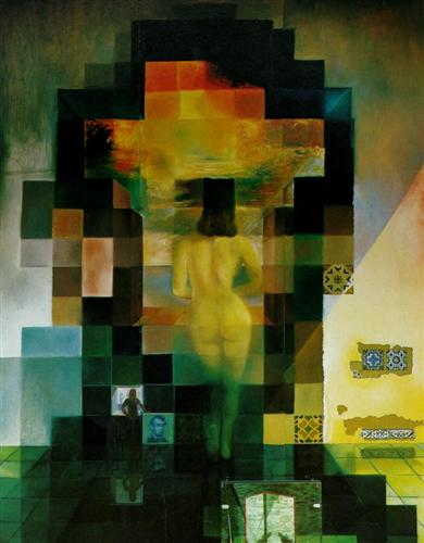
Original Image

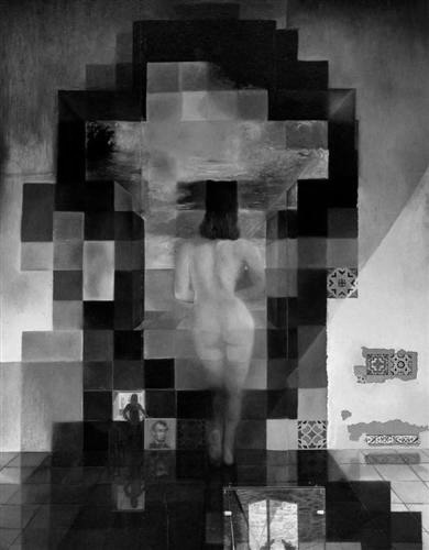
Gaussian Stack

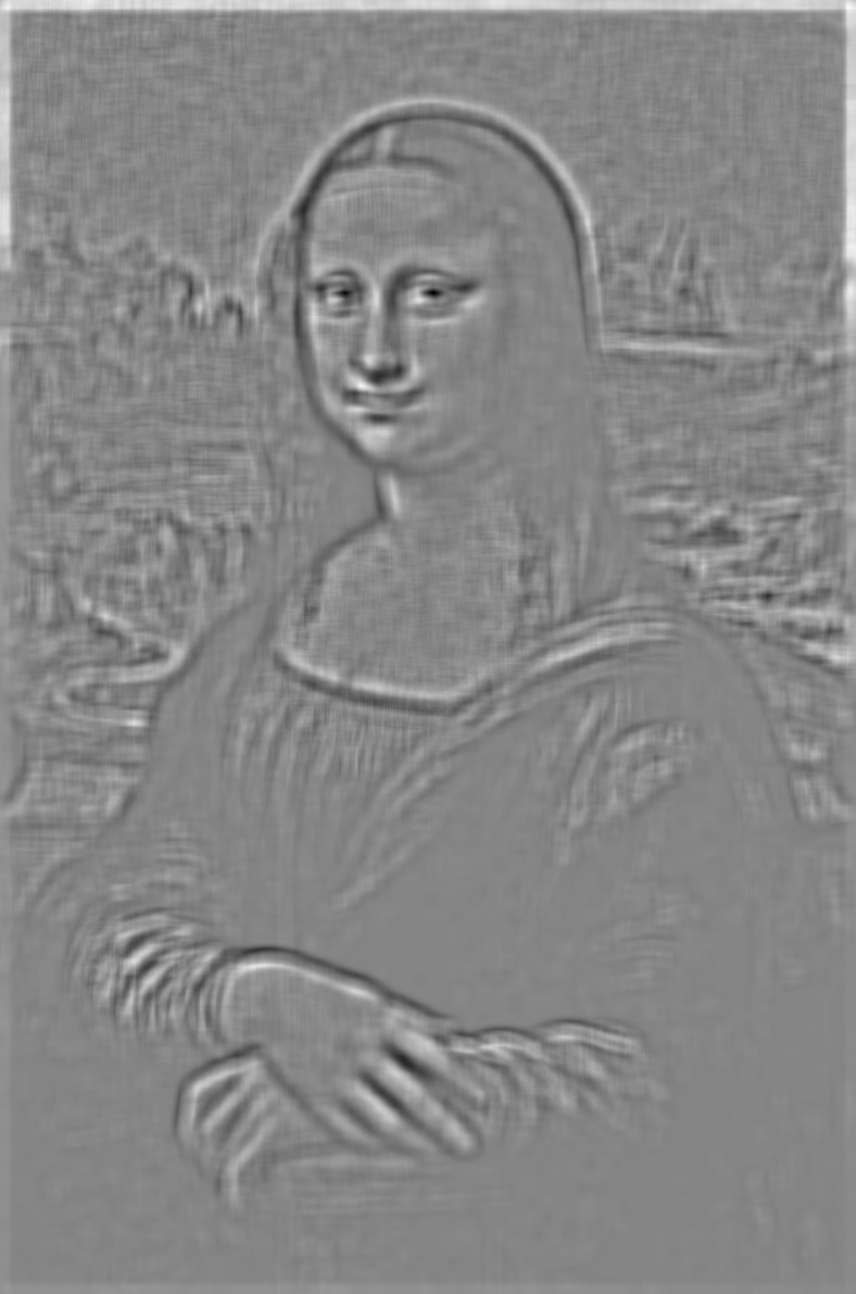
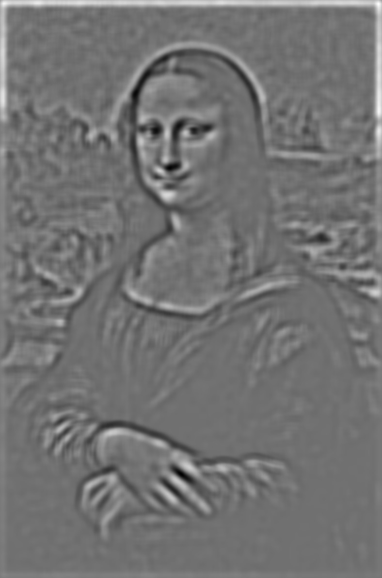
Laplacian Stack

Original Image

Gaussian Stack

Laplacian Stack

Original Image

Gaussian Stack

Laplacian Stack

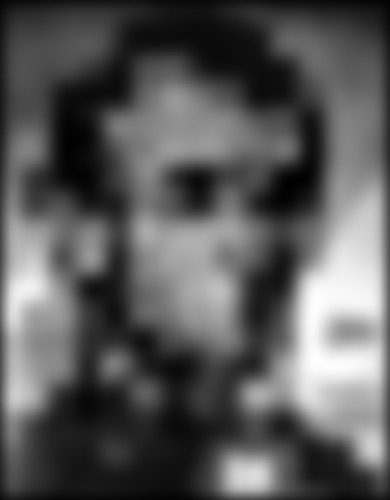
Now, we can apply this procedure to the Mark Zuckerberg image from Part 1.2 above.

Original Image

Gaussian Stack

Laplacian Stack

Part 1.4: Multiresolution Blending

This algorithm was implemented by calculating a mask for the two images, then calculating the Laplacian stack for each input image and a Gaussian stack for the mask. Then, we initialize an output matrix, and for each level of the stacks, we mask each result from the Laplacian stack with the corresponding entry in the corresponding mask’s Gaussian stack. These masked results are then added to the output matrix. At the end, the output matrix is normalized by N, the depth of all of the stacks. For color images, this is done separately for each channel and the channels are then recombined.

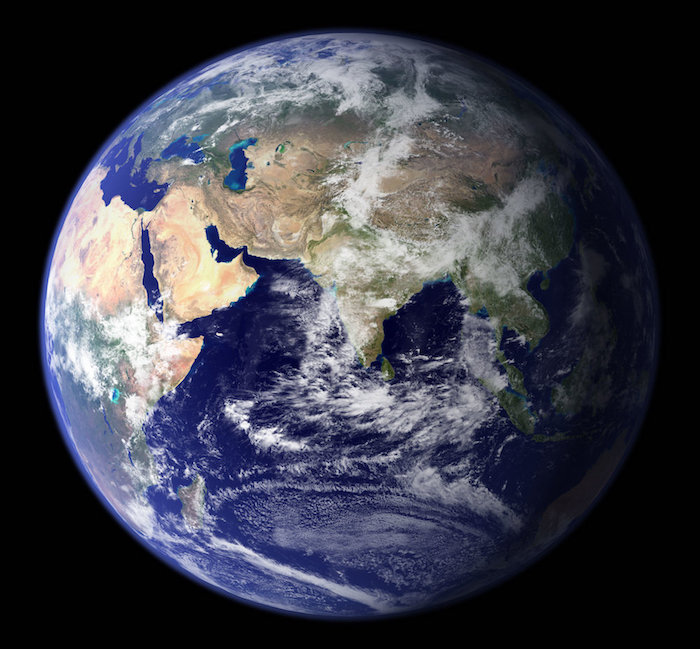
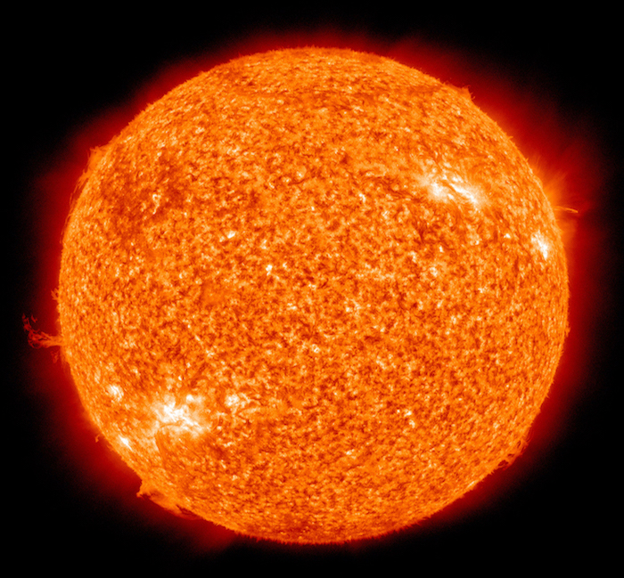
Original Images

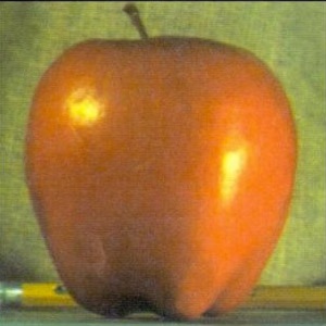
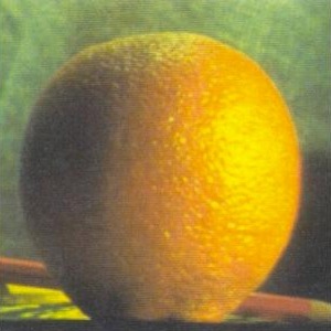
Blended Image

(mask: horizontal, stack depth: 5, mask Gaussian size: 31, mask Gaussian sigma: 25, Laplacian stacks size: 21, Laplacian stacks sigma: 1.0)

Original Images

Blended Image

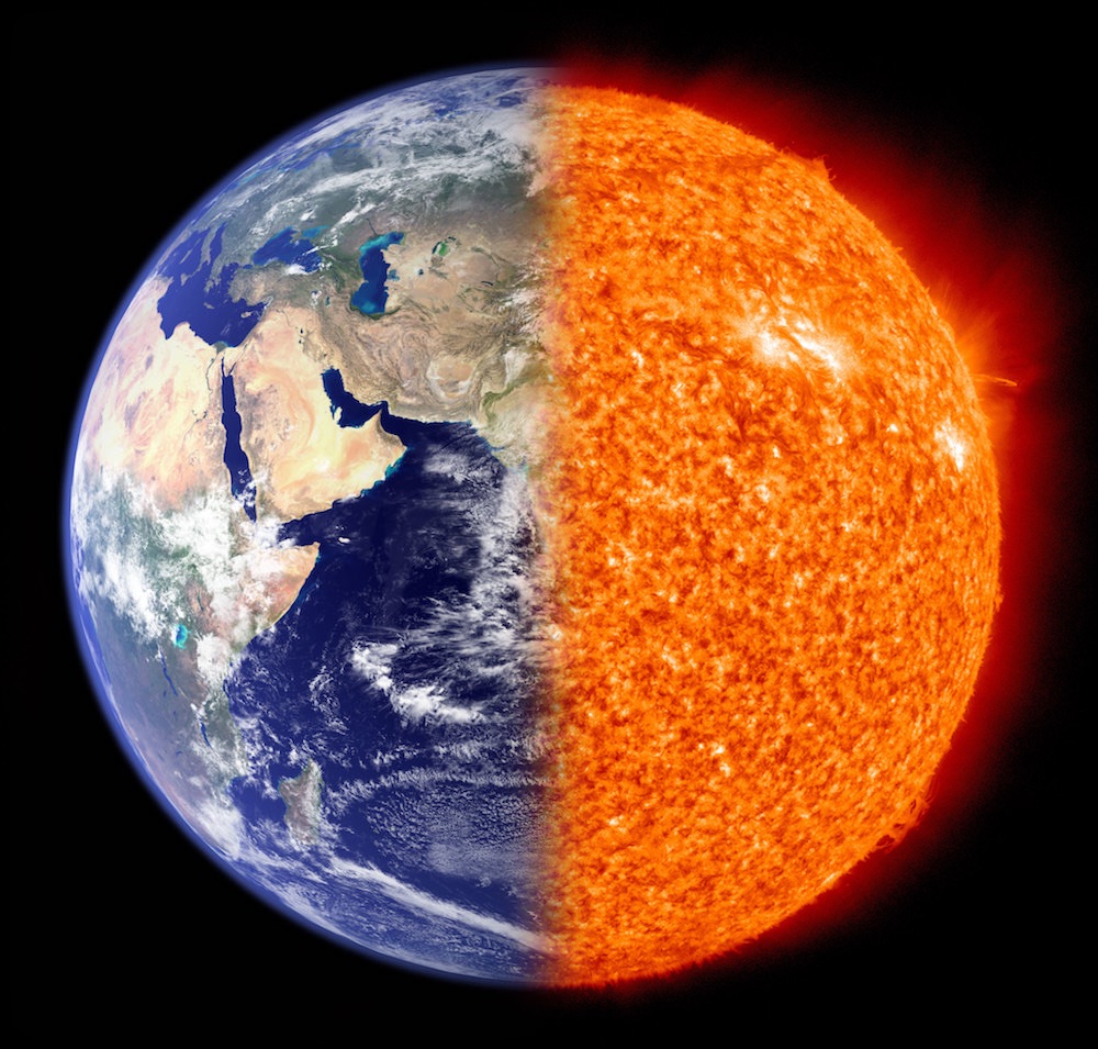
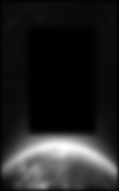
The rare EarthSun makes an appearance.

(mask: vertical, stack depth: 5, mask Gaussian size: 31, mask Gaussian sigma: 25, Laplacian stacks size: 21, Laplacian stacks sigma: 1.0)

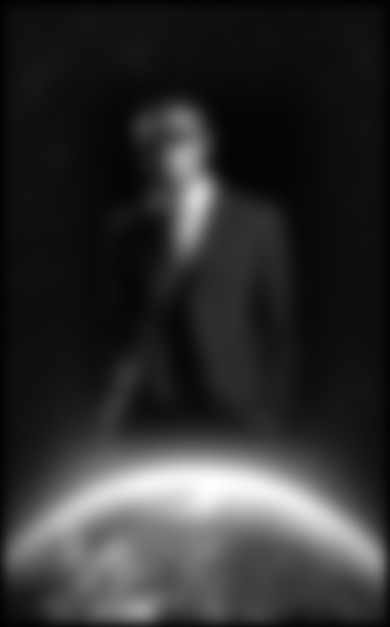
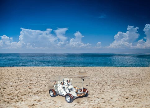
Original Images

Blended Image

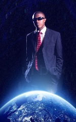
This man is hovering over the horizon!

(mask: irregular, stack depth: 5, mask Gaussian size: 31, mask Gaussian sigma: 25, Laplacian stacks size: 21, Laplacian stacks sigma: 1.0)

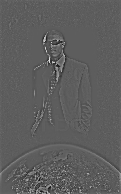
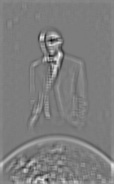
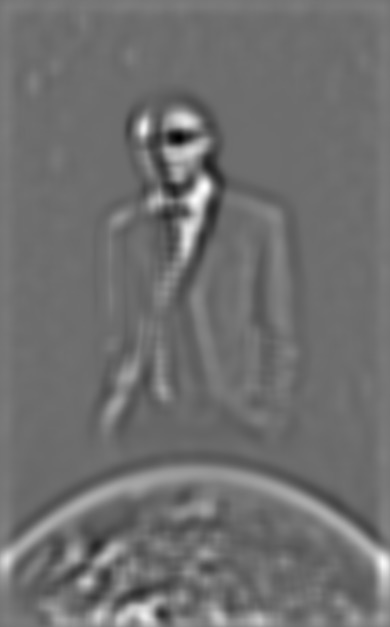
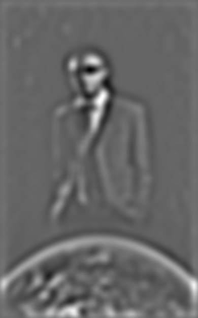
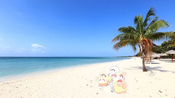
We can analyze this image with Laplacian stacks over the blended image and the two masked source images. These stacks all use a filter size of 15 and sigma of 15.

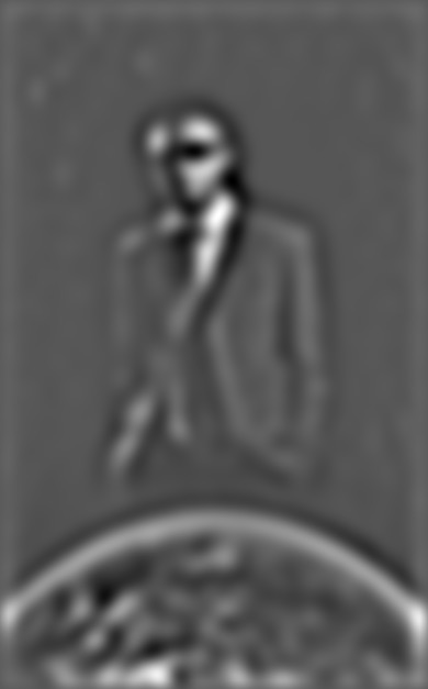
Source Image 1 Laplacian

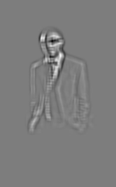
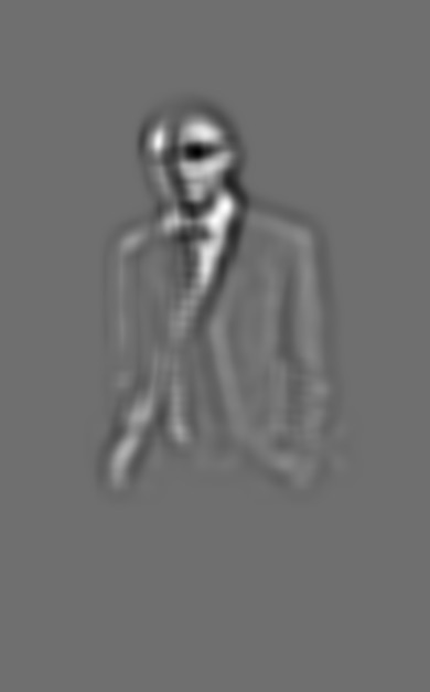
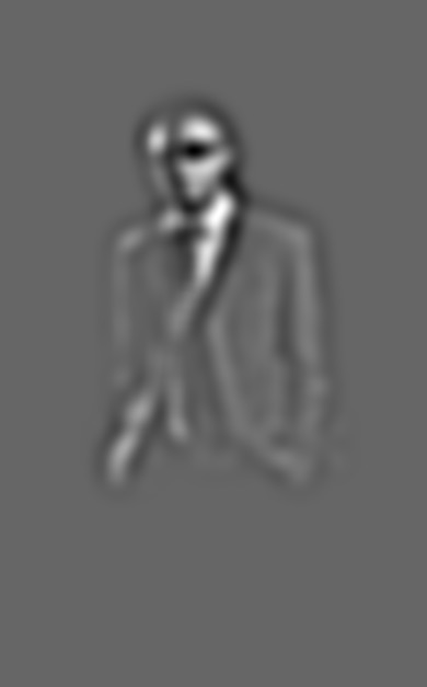
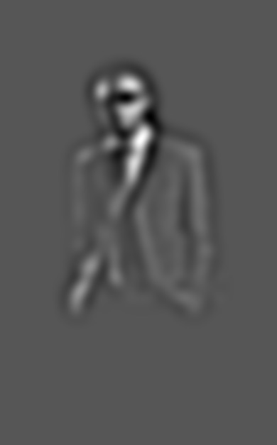
Source Image 2 Laplacian

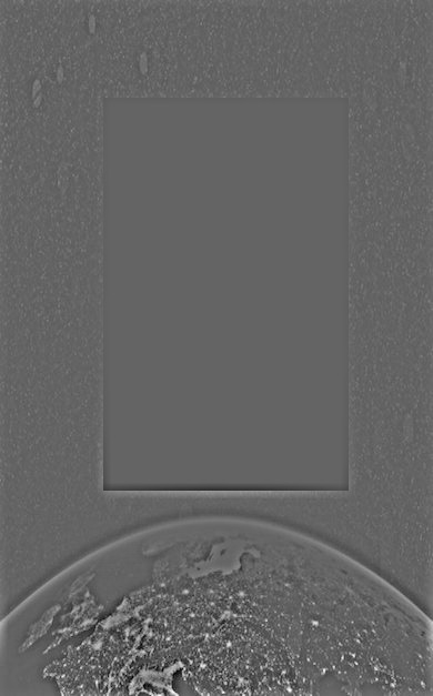
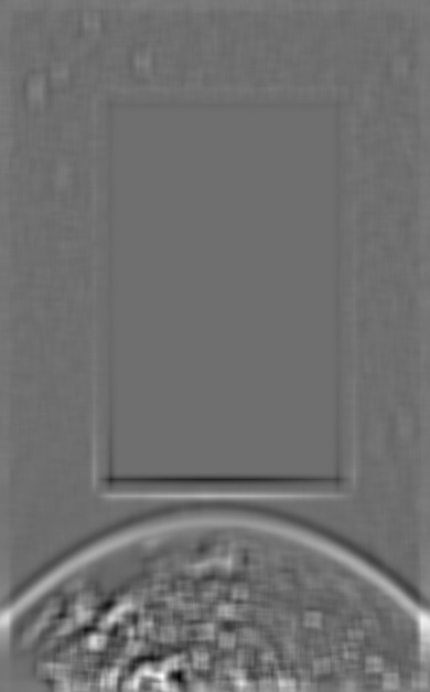
Blended Image Laplacian

Part 2.1: Toy Problem

I solved the toy problem according to the given equation and instructions. The source image and result image are below, note that they are the same.

Original Image

Solved Image

Part 2.2: Poisson Blending

First, it is important to rescale each color channel of the source image s and the target image t to proportionately spread the pixel values across the range of 0 to 1, so the least squares solver is working with gradients and pixel values of the same magnitude. Then, we build a least-squares matrix of the desired result gradients from source image s, filling in the edge constraints whenever we hit an edge of the mask. I then ran this matrix through a sparse least squares solver to obtain the best values for the pixels being masked into the final image v, and then filled them in. The rest of the pixels were then copied from the target image t. For color images, this process was repeated independently once per color channel, then the channels were combined to obtain the final image.

Favorite Result

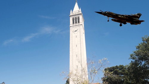
A sonic jet blast echoes across the campus…

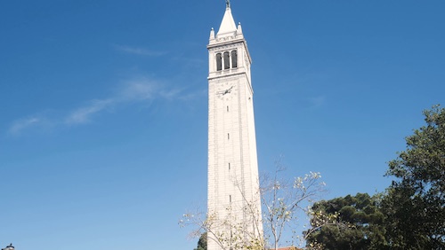
Target Image t

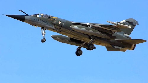
Source Image s

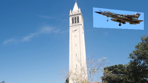
Direct Pixel Copy

This image worked using the standard method described above. Notably, the plane in the image became extremely washed out after processing when the rescaling step described above was not used, but after adding this functionality the image quality improved dramatically to the results we see above.

We now present additional results below.

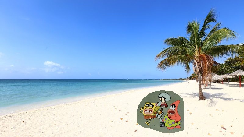
This is a failure case: the texture of the source image s was just too different from the surrounding texture of t. So even though the color could be matched, it still does not look good.

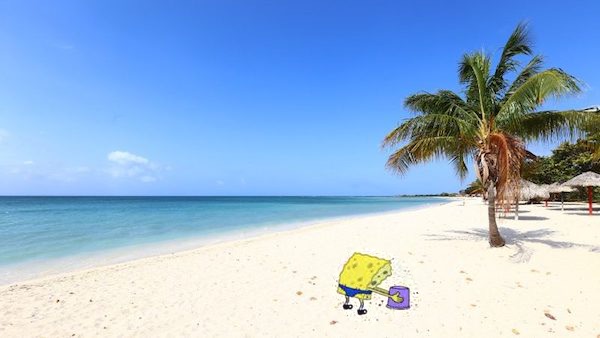
This is also a failure case: the background color of the source image s was much darker than the surrounding texture of t, so the pixels that least squares solved became extremely washed out. Although a failure case, this result shows an interesting look into how the algorithm works. For comparison, the direct copy image is below.

Direct copy version of the above image transfer.

Something’s off here…

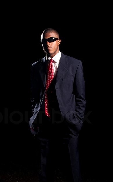
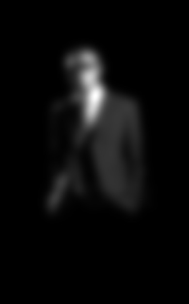
We can also compare the results from Poisson and Laplacian blending. Using these images from below, we can display the Laplacian and Poisson results to compare the methods.

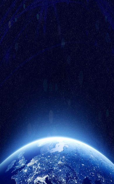
Target Image t

Source Image s

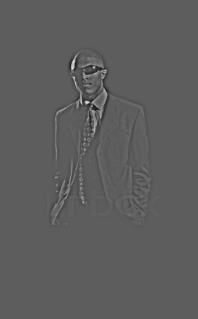
Laplacian Blended Image

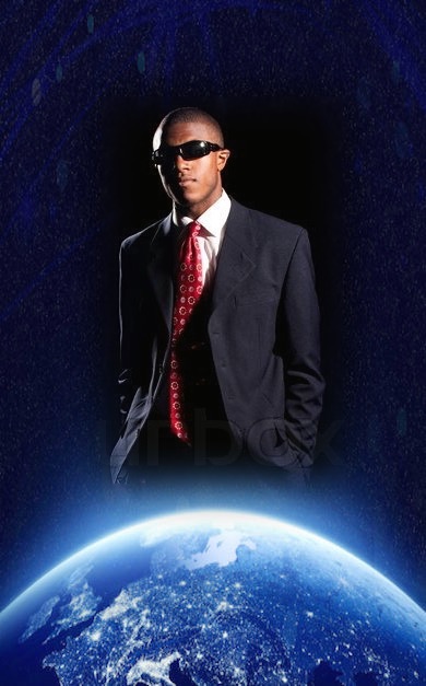
Poisson Blended Image

It seems that the Poisson method works better for this image, mainly because of the glowing blue gradient. On the Poisson image, this blue color is carried through onto the solved pixel values v very nicely, whereas the Laplacian blended image does not allow this gradient to overlay a large portion of the man in the suit. Instead, this blue portion only shows in the feathered section. On the other hand, the Laplacian image was much faster to calculate, and we were able to calculate a higher resolution image as a result, so there is some value in that method. In fact, producing an image of the resolution as the Laplacian method but with the Poisson method would have taken an order of magnitude longer than the Laplacian result. As a result, if computation time is not a concern, then the Poisson blending method is definitely preferred for this pair of images. Otherwise, the Laplacian method produces a very good result with much less computation, so it may be preferred.