Fun with Frequencies and Gradients
CS194-26 Fall 2018
Andrew Campbell, cs194-26-adf
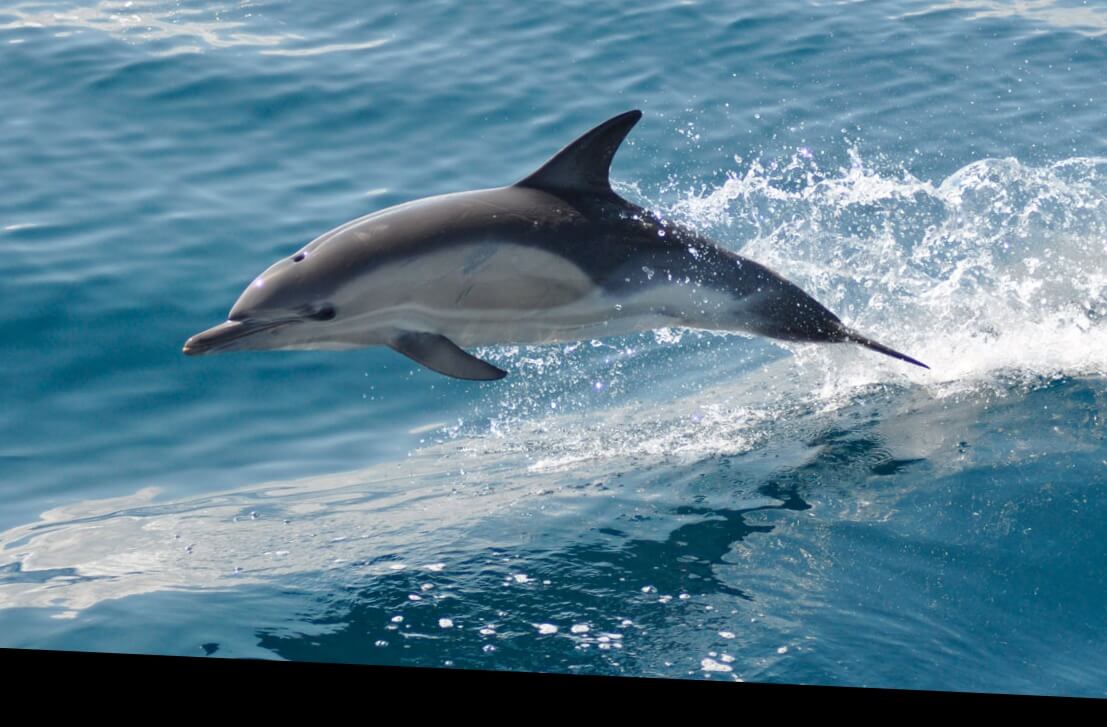
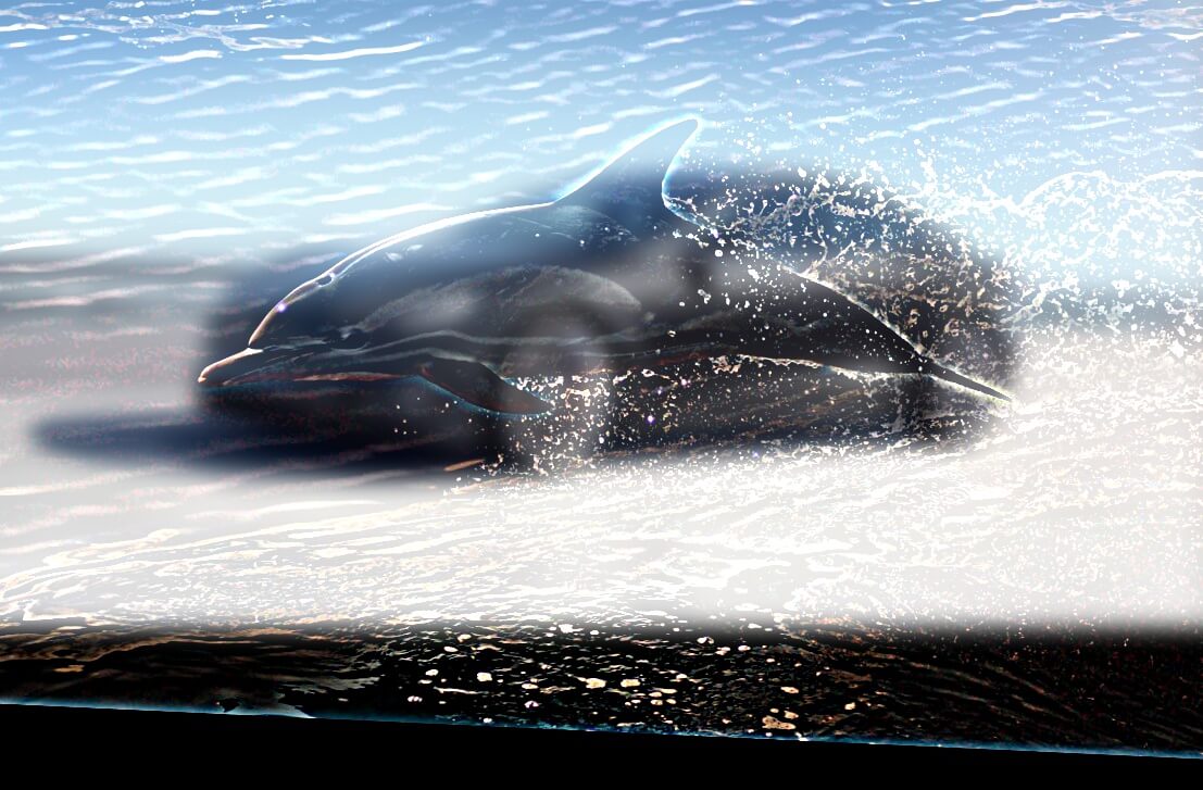
Part 1.1: Sharpening
Unsharp Masking Filter
The unsharp masking filter, contrary to it’s name, is a common algorithm for sharpening an image. It works by utilizing a slightly blurred version of the original image which is then subtracted away from the original to detect the presence of edges, creating the unsharp mask (effectively a high-pass filter). By adding the mask back to the original image, contrast is selectively increased along the edges, leaving behind a sharper final image.
A simple Gaussian blur suffices for the blurred image; I used a \( 9 \times 9 \) Gaussian kernel with \( \sigma = 10 \). Using \( \alpha = 0.5 \), here are some of the before-and-after results:


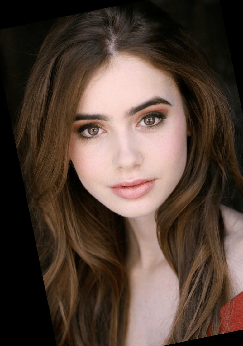
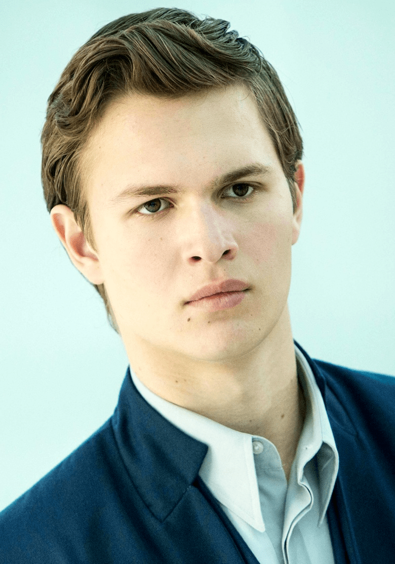
Part 1.2: Hybrid Images
Background
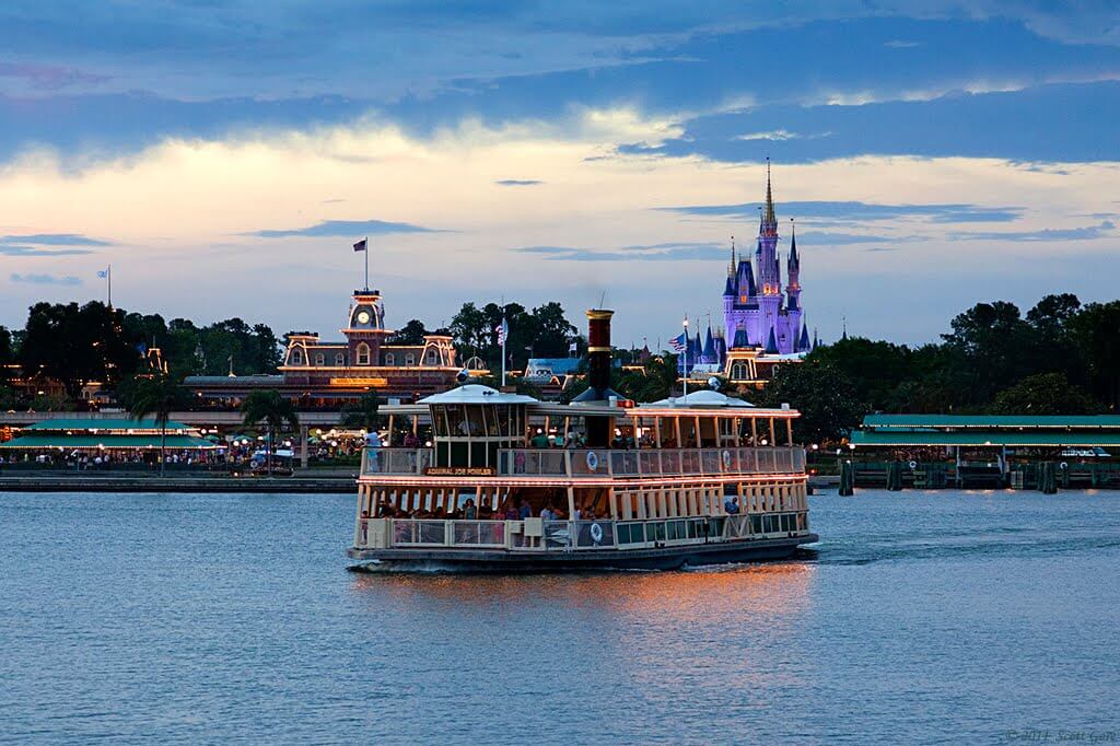
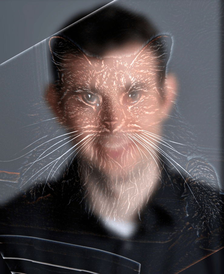
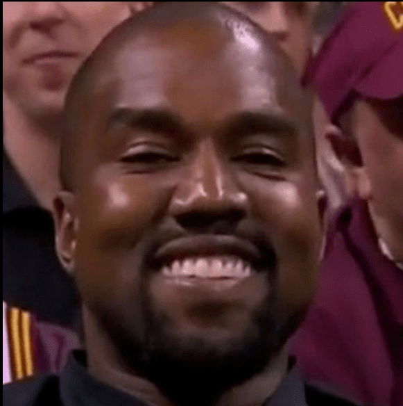
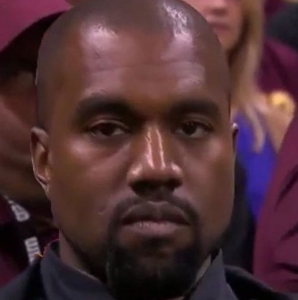
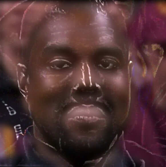
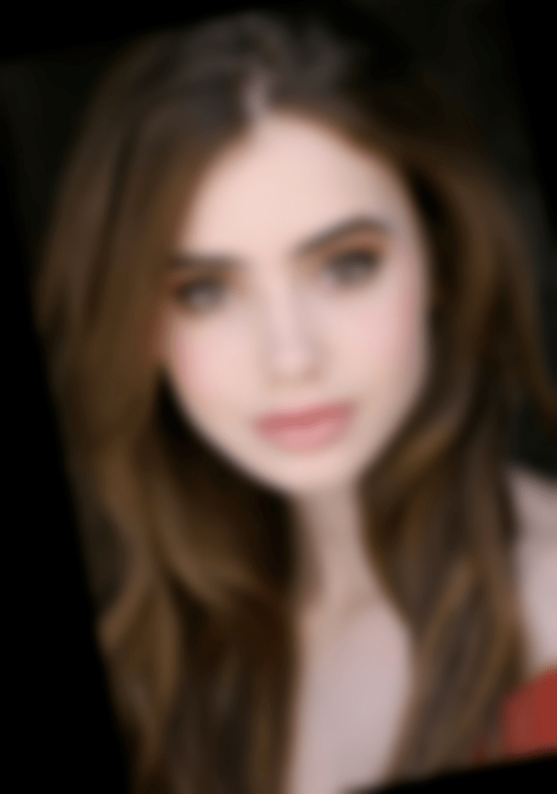
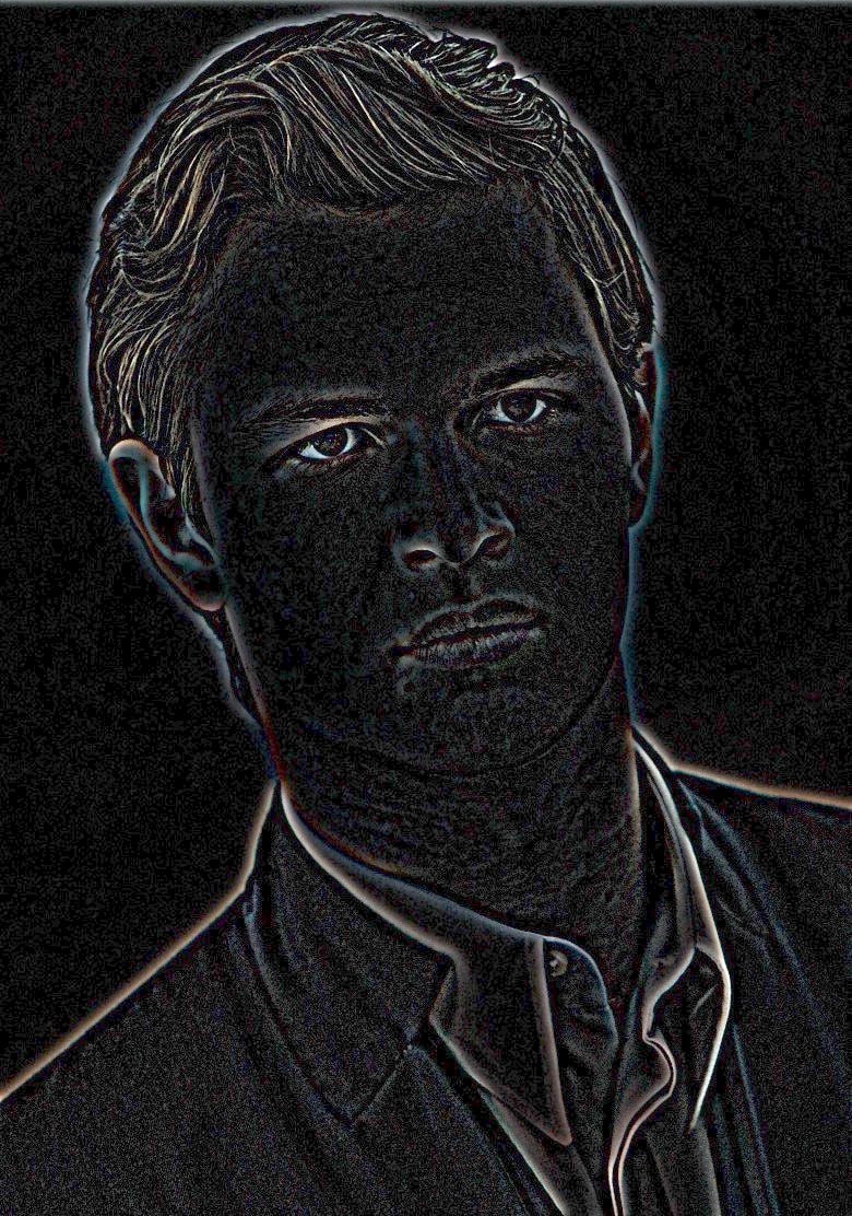
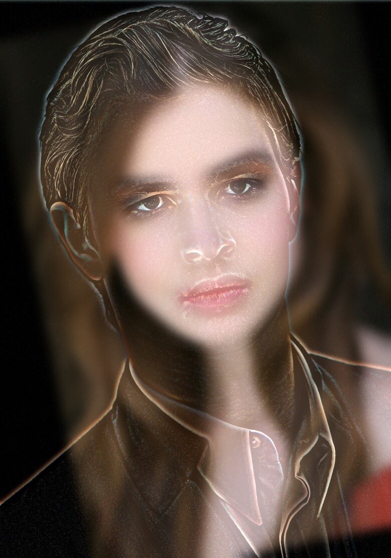
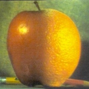
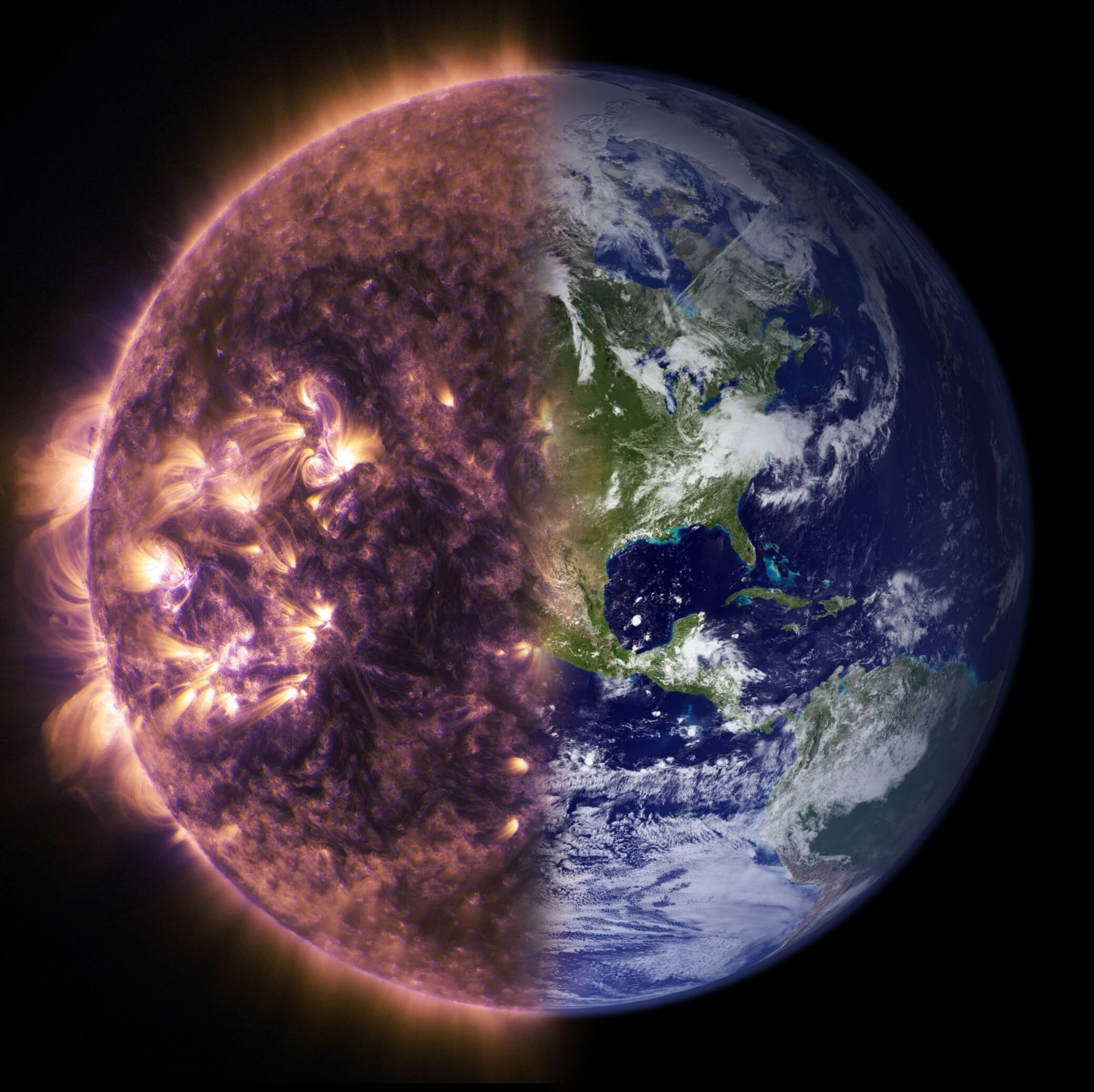
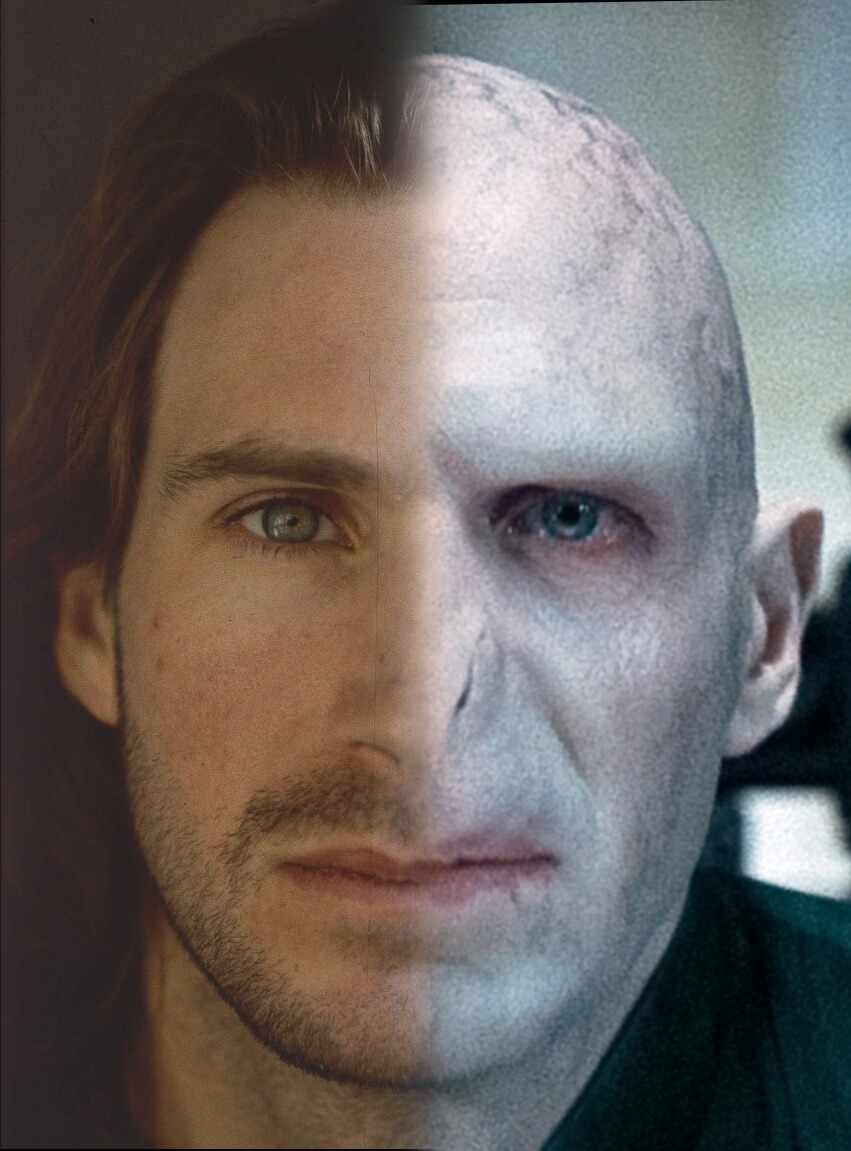
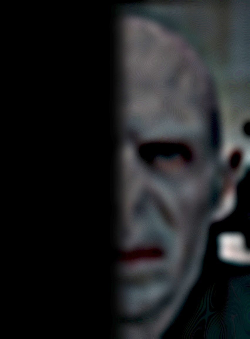
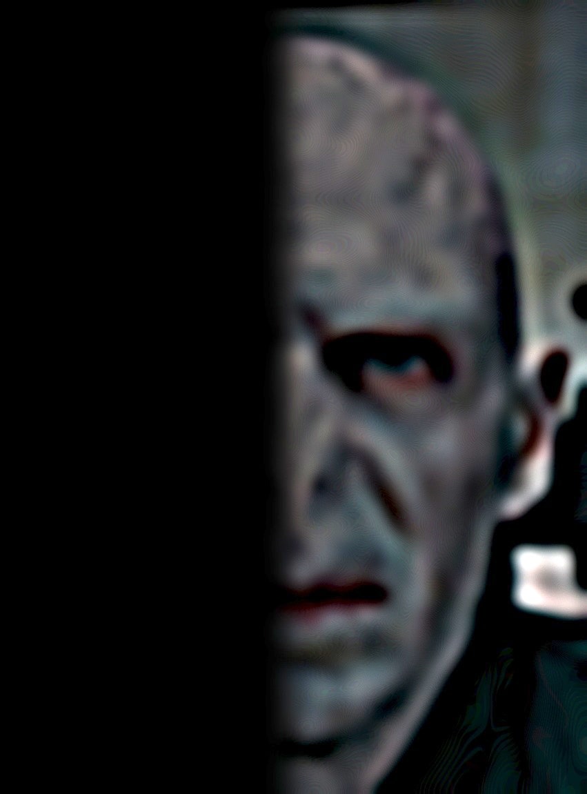
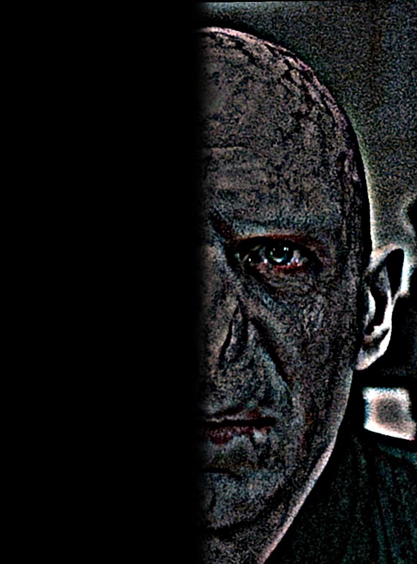
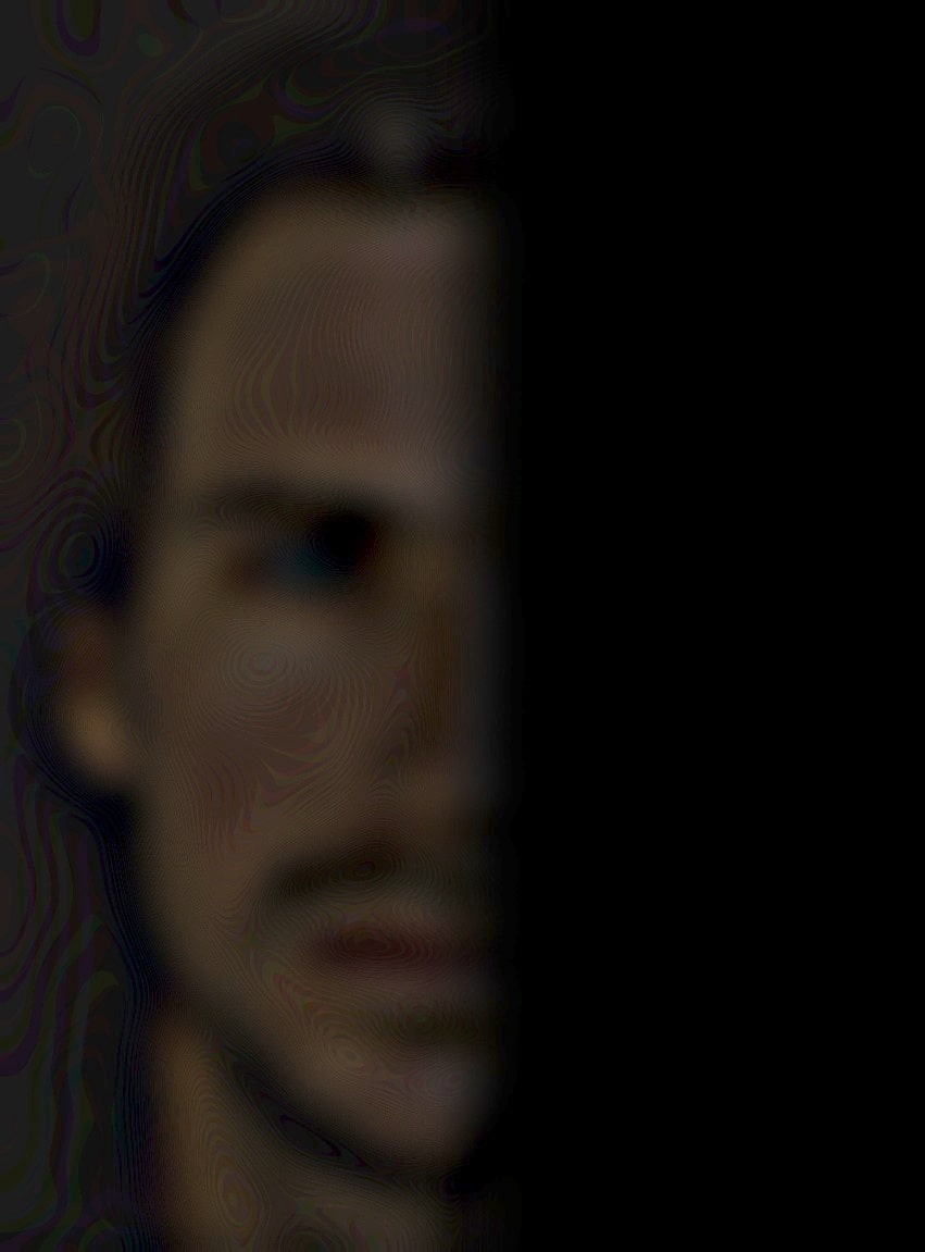
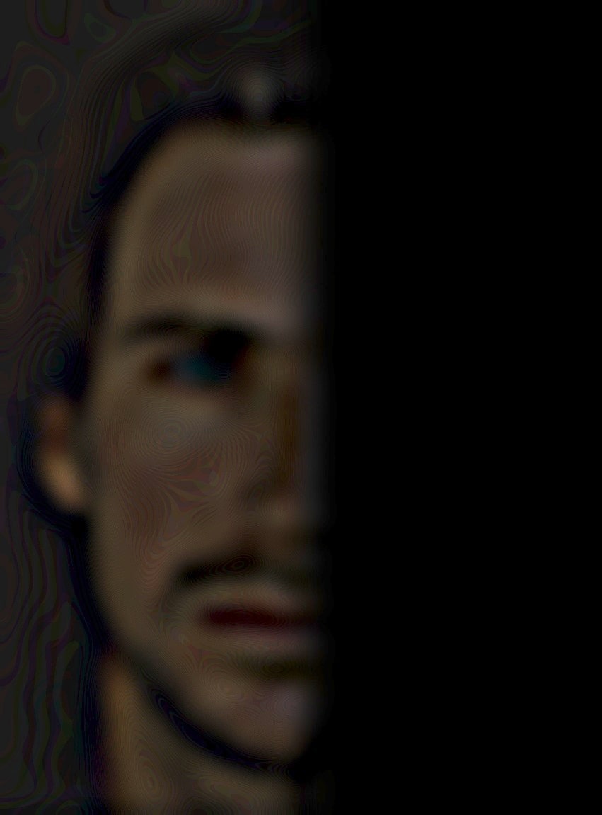
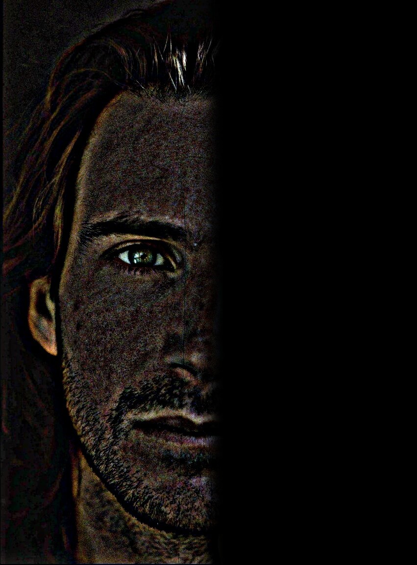
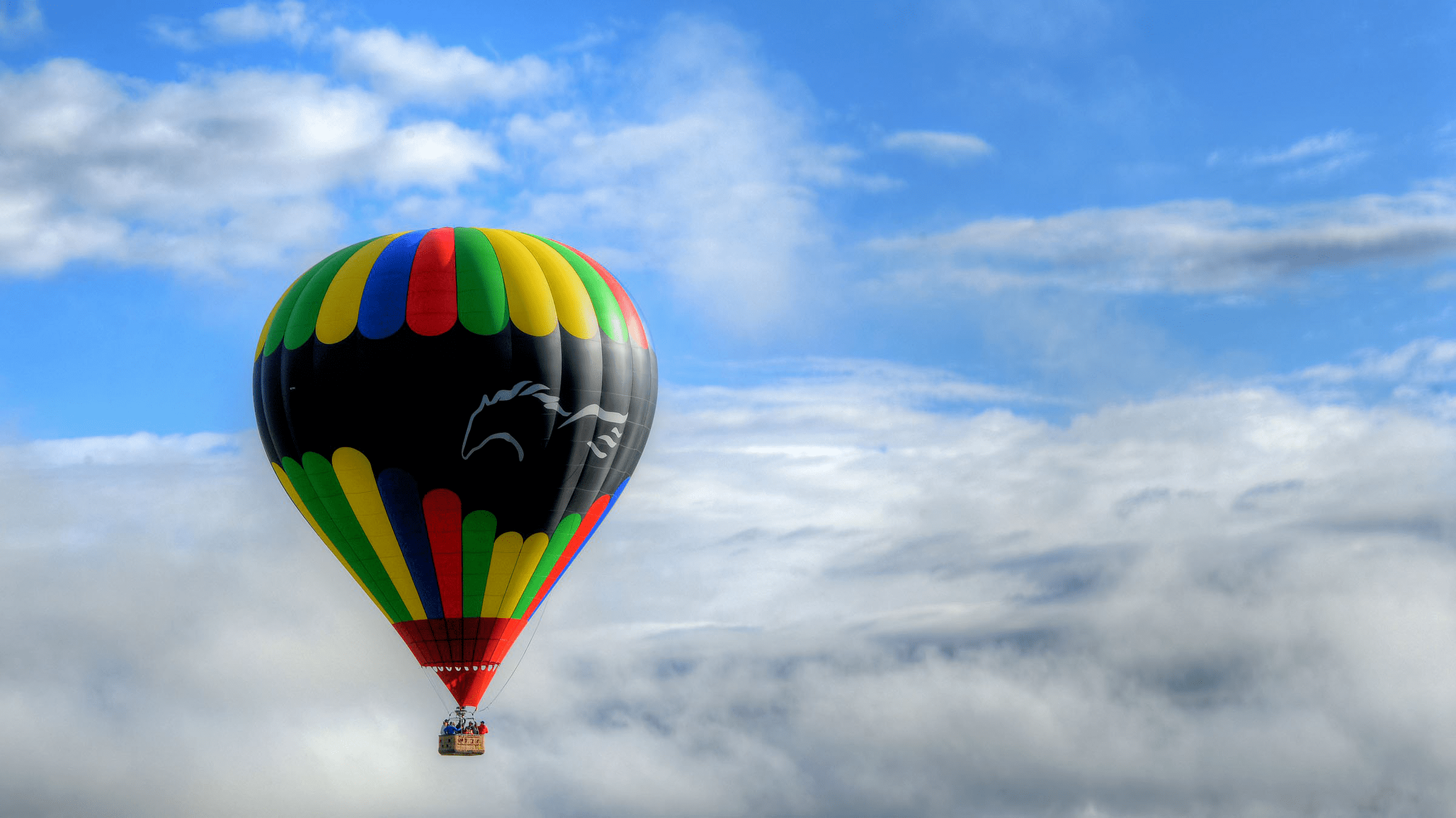
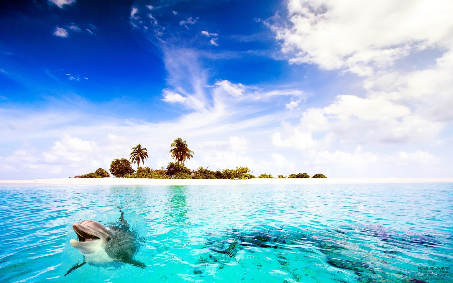
Hybrid images are static images that change in interpretation as a function of the viewing distance. The basic idea is that high frequency tends to dominate perception when it is available, but, at a distance, only the low frequency (smooth) part of the signal can be seen. By blending the high frequency portion of one image with the low-frequency portion of another, you get a hybrid image that leads to different interpretations at different distances.
Implementation
We begin by finding pairs of images we want to turn into hybrid images and aligning on 2-point correspondences, e.g. eyes. To low-pass filter one image, we simply apply a Gaussian blur. To high-pass filter the other image, we subtract the Gaussian-filtered image from the original (this is the same idea as the unsharp filter discussed above).
The Gaussian kernel sizes used to create the low-pass and high-pass filter determine the low-frequency-cutoff and the high-frequency-cutoff, respectively. Through some experimentation I found that 35 worked well for the high-frequency-cutoff and 61 worked well for the low-frequency-cutoff. I again used \( \sigma = 10 \) for the kernels.
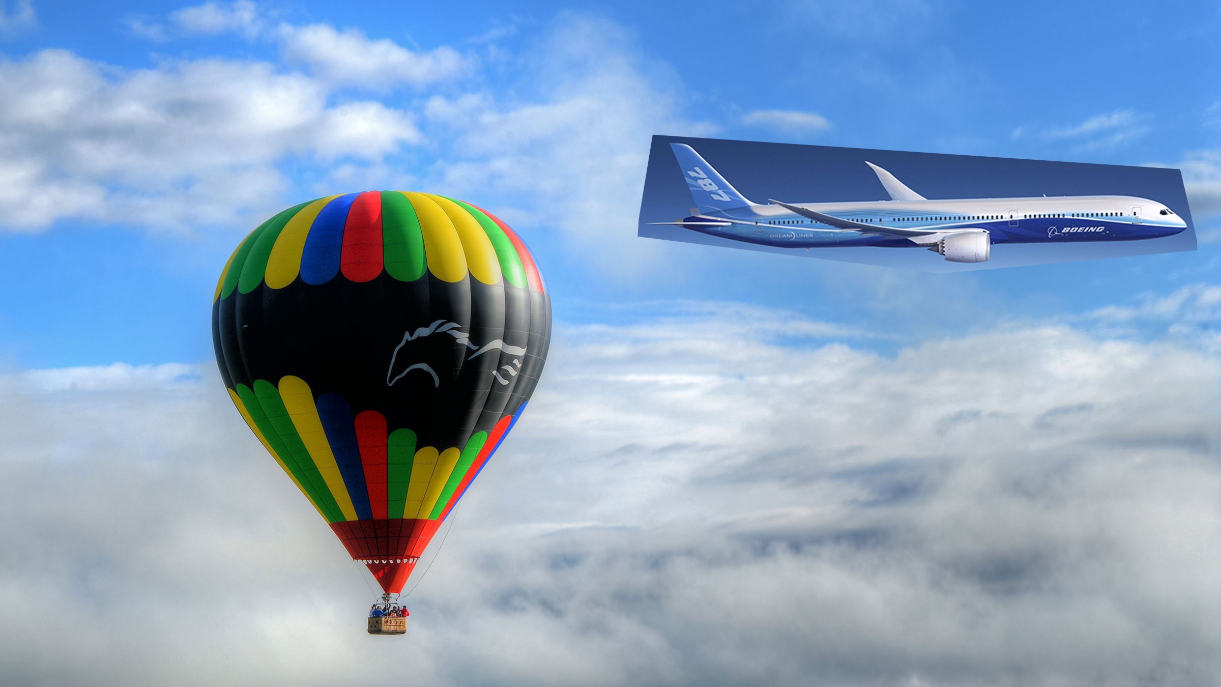
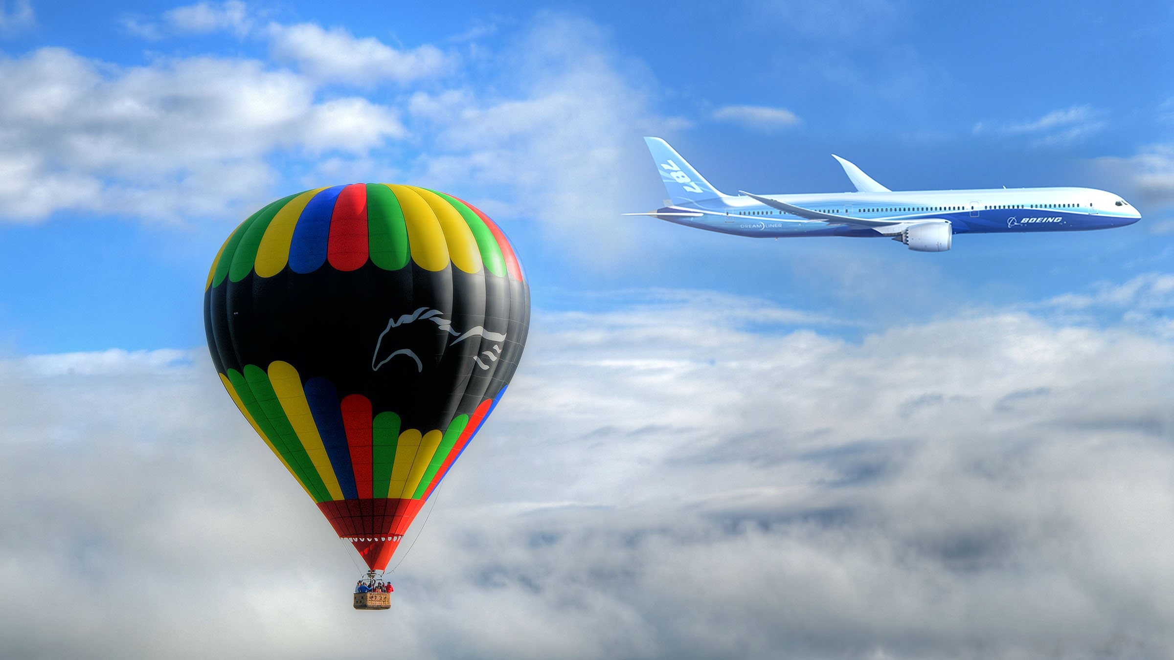
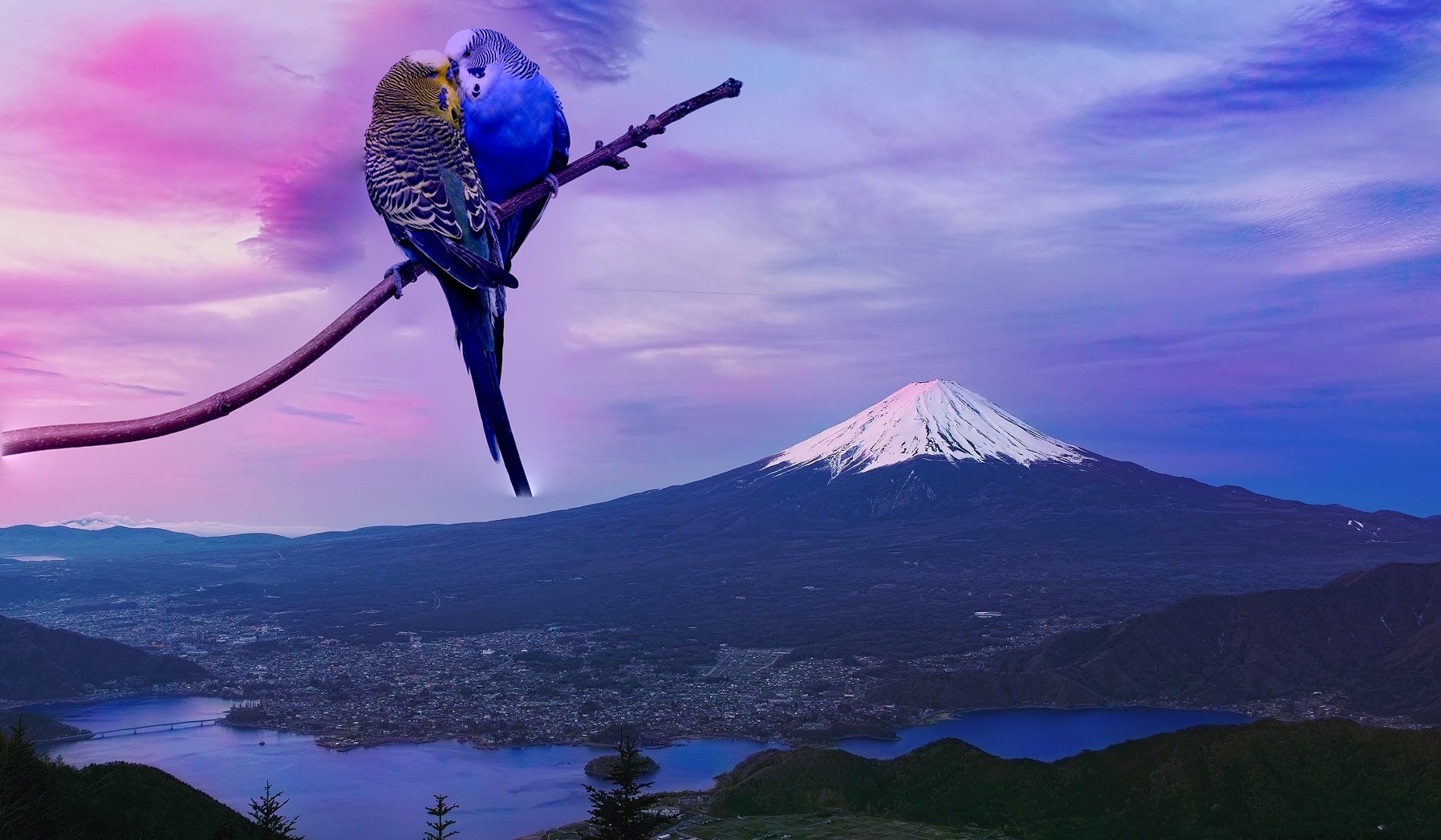
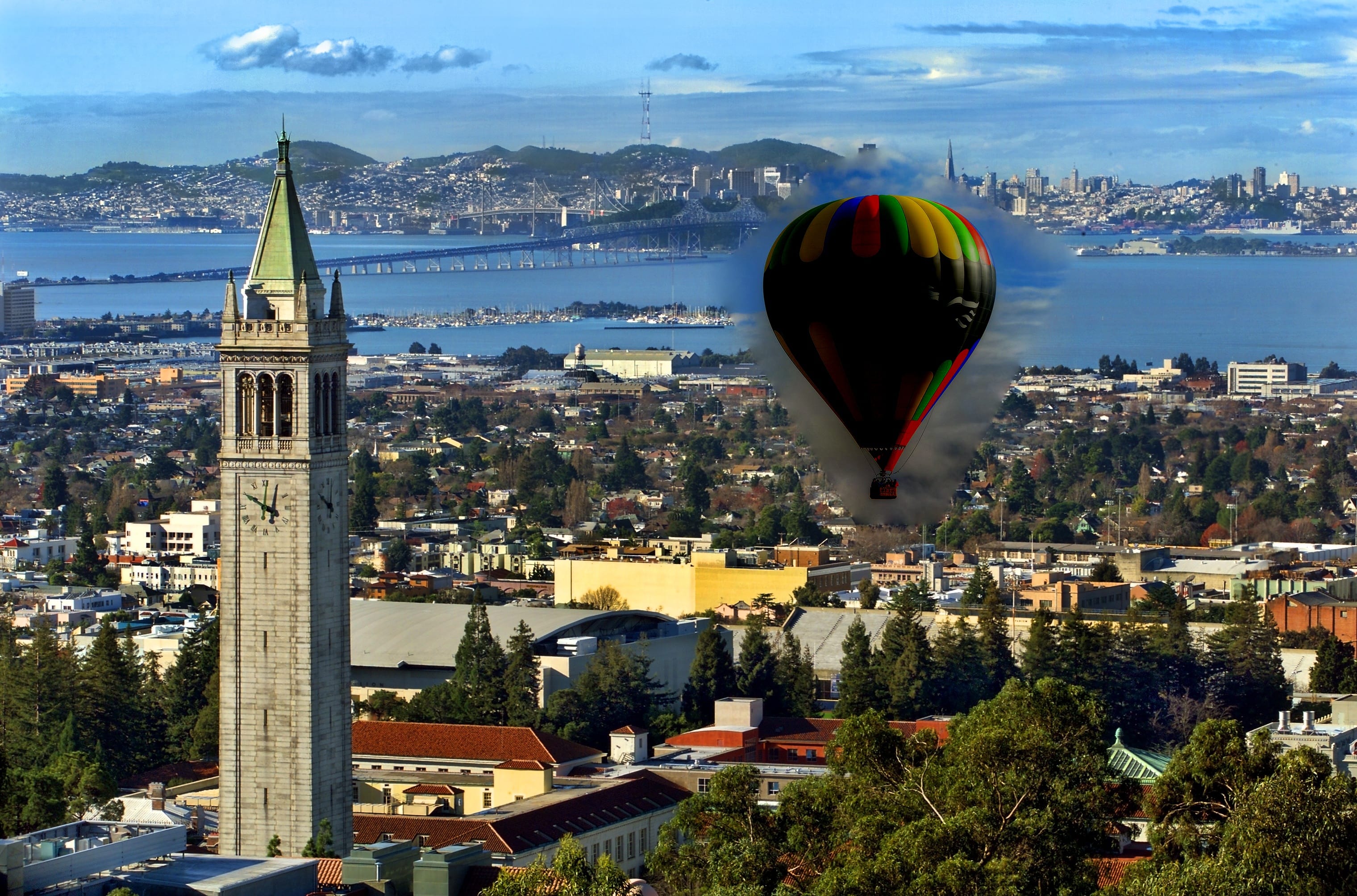
Lastly we simply add the two images. I kept color in both the low-pass and high-pass images and thought the result looked good. Here are some of the results; for maximum effect, look at the images from both close-up and far-away and see how your perception changes.
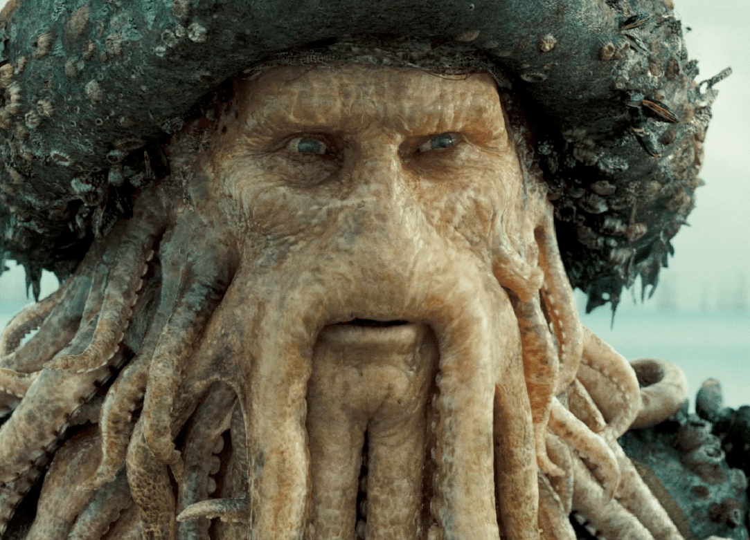


Not all pairings were quite so successful:

The images should ideally have similar features and be of similar shape for the best effect.
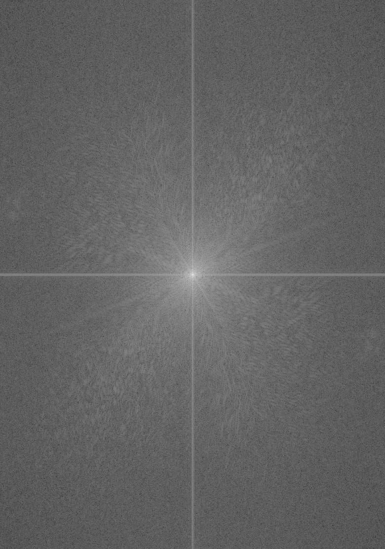
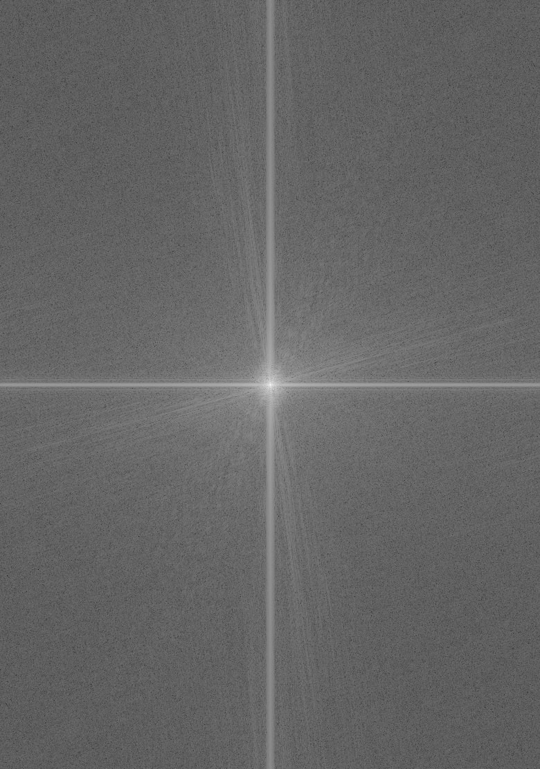
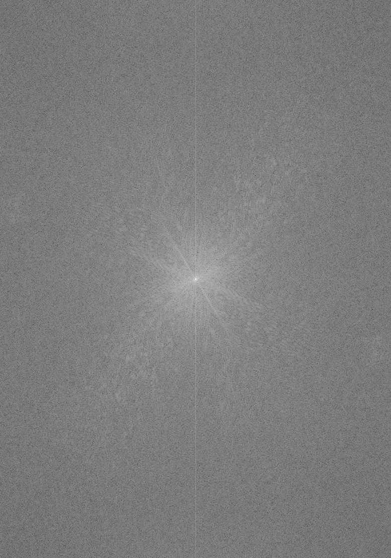
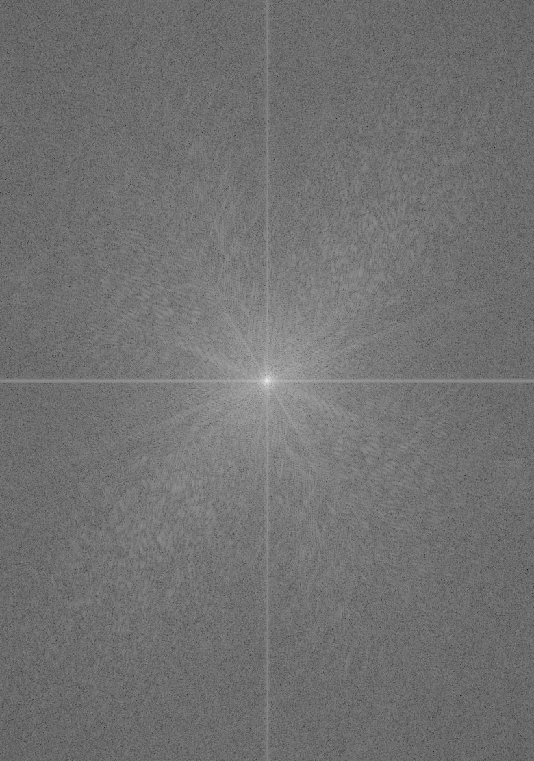
Frequency analysis
Here we illustrate the process by showing the log magnitude of the Fourier transform of the two input images, the filtered images, and the hyrbid image, respectively.

Part 1.3: Gaussian and Laplacian Stacks
An image pyramid is a multi-scale signal representation of an image in which an image is subject to repeated smoothing and subsampling. An stack is similar to a pyramid, but without the downsampling.
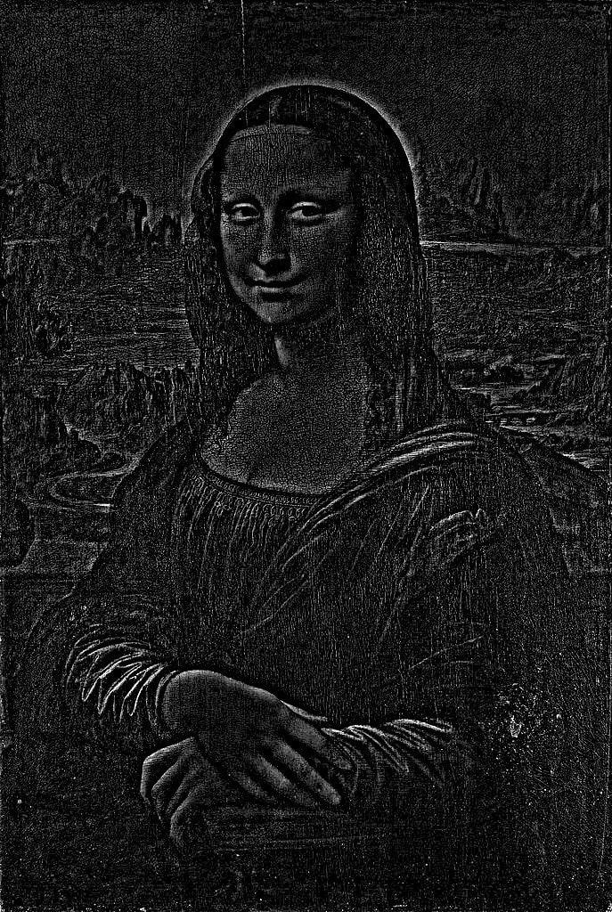
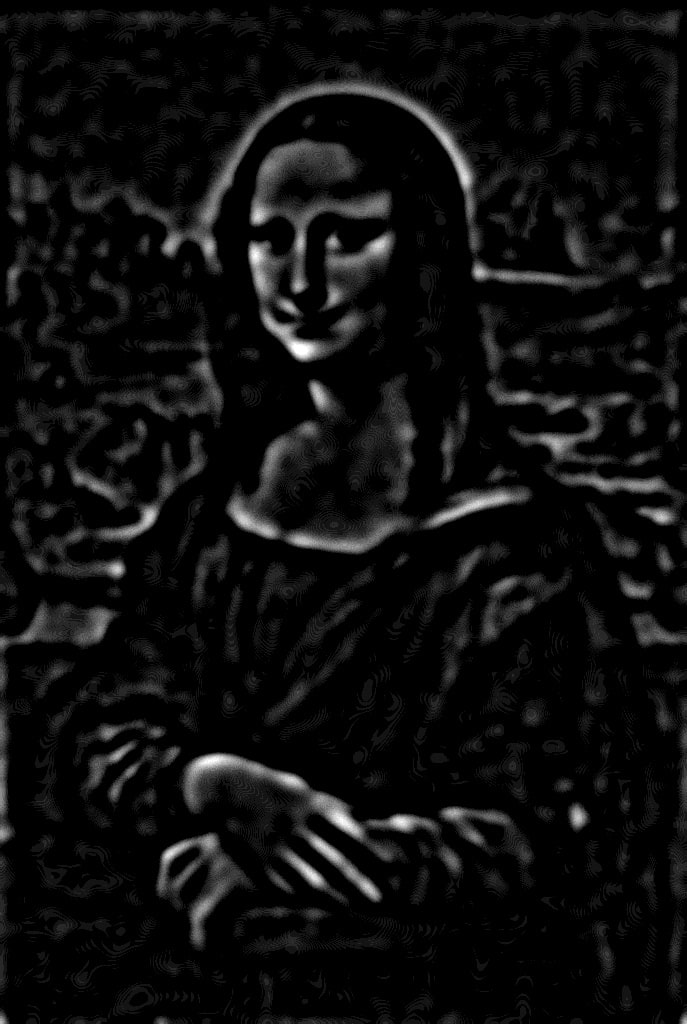
In a Gaussian stack, subsequent images are weighted down using a Gaussian blur. A Laplacian stack is constructed from a Gaussian stack: each layer stores the difference between the corresponding Gaussian layer and the level above it (the first level is the difference between the original image and first level Gaussian).
By visualizing the Gaussian and Laplacian stacks for images that contain structure in multiple resolutions, we can extract the structure at each level. Shown below are the Gaussian stacks (top) and Laplacian stacks (bottom) for some interesting images.
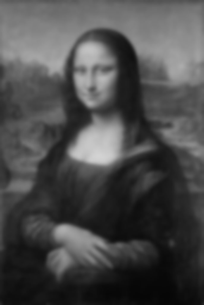
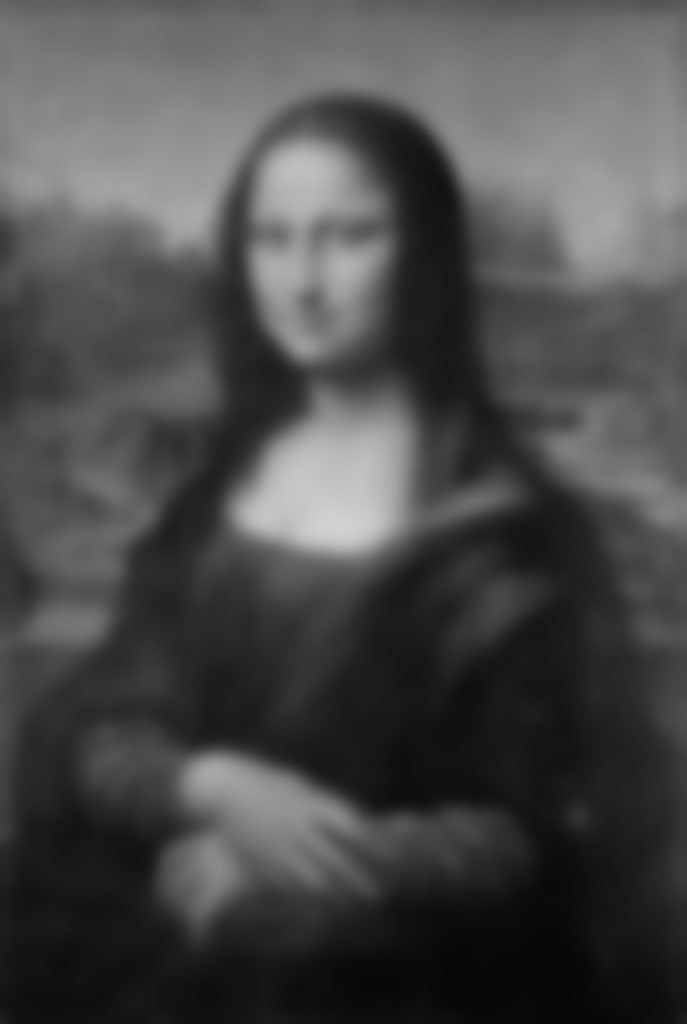
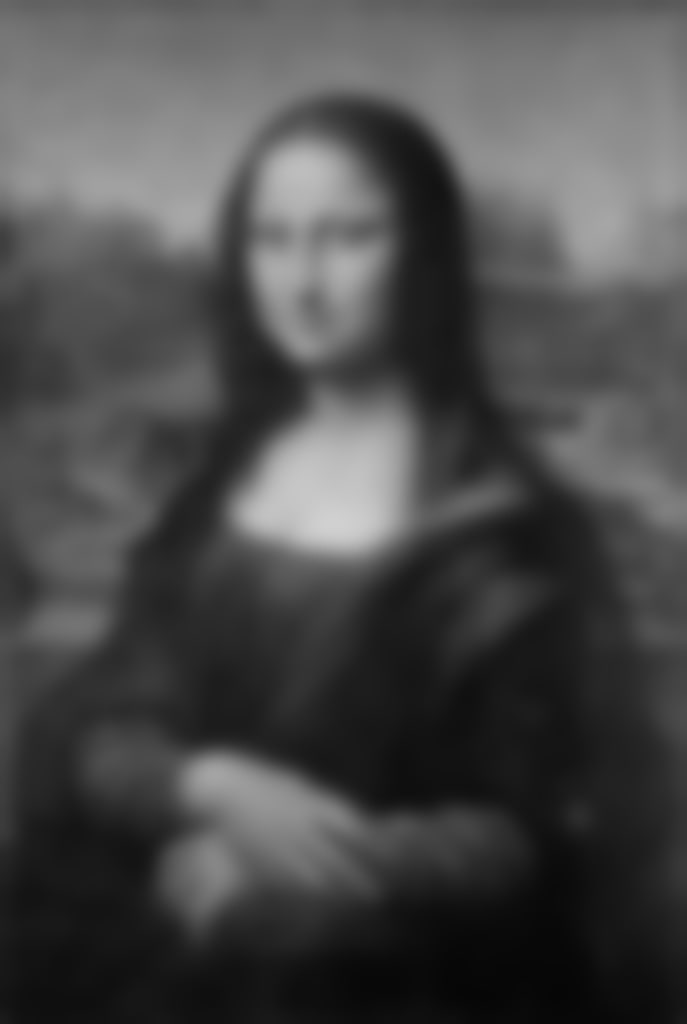


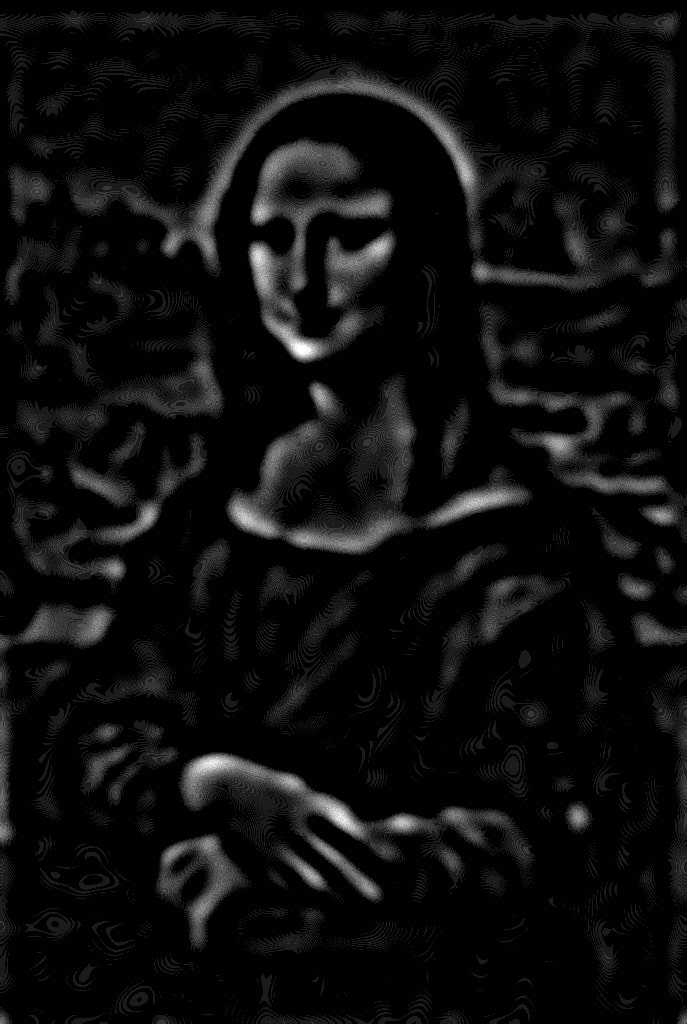

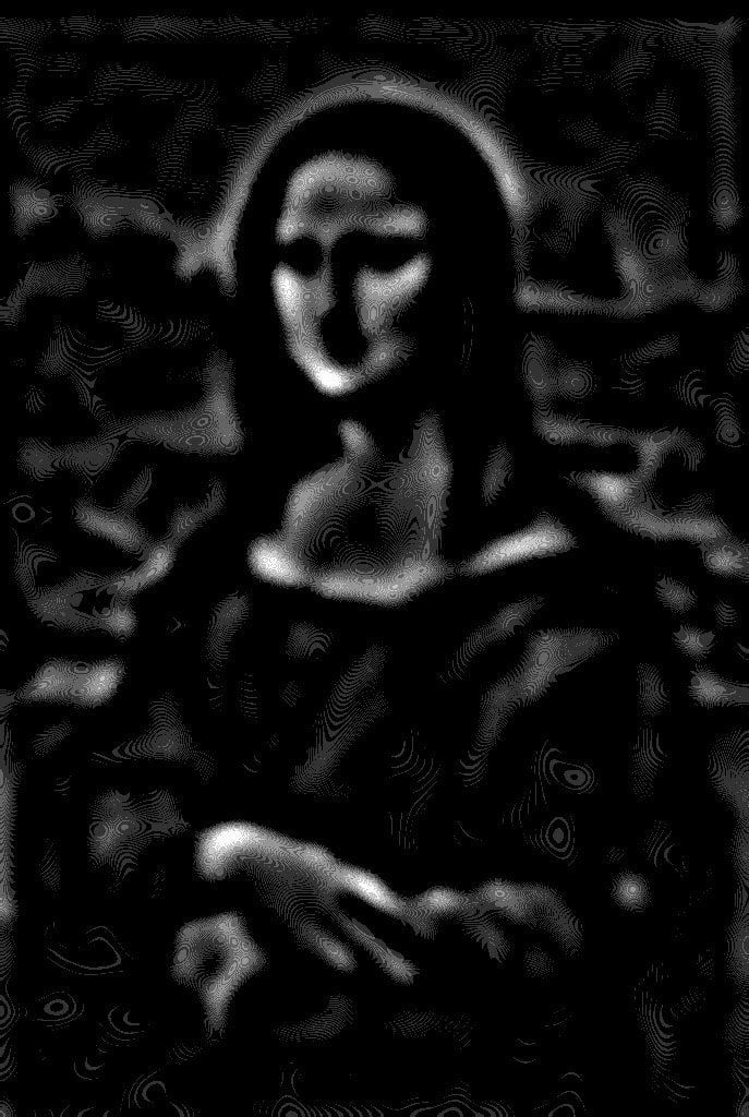
Notice the Mona Lisa’s smile does not appear until we filter out the high-frequencies.
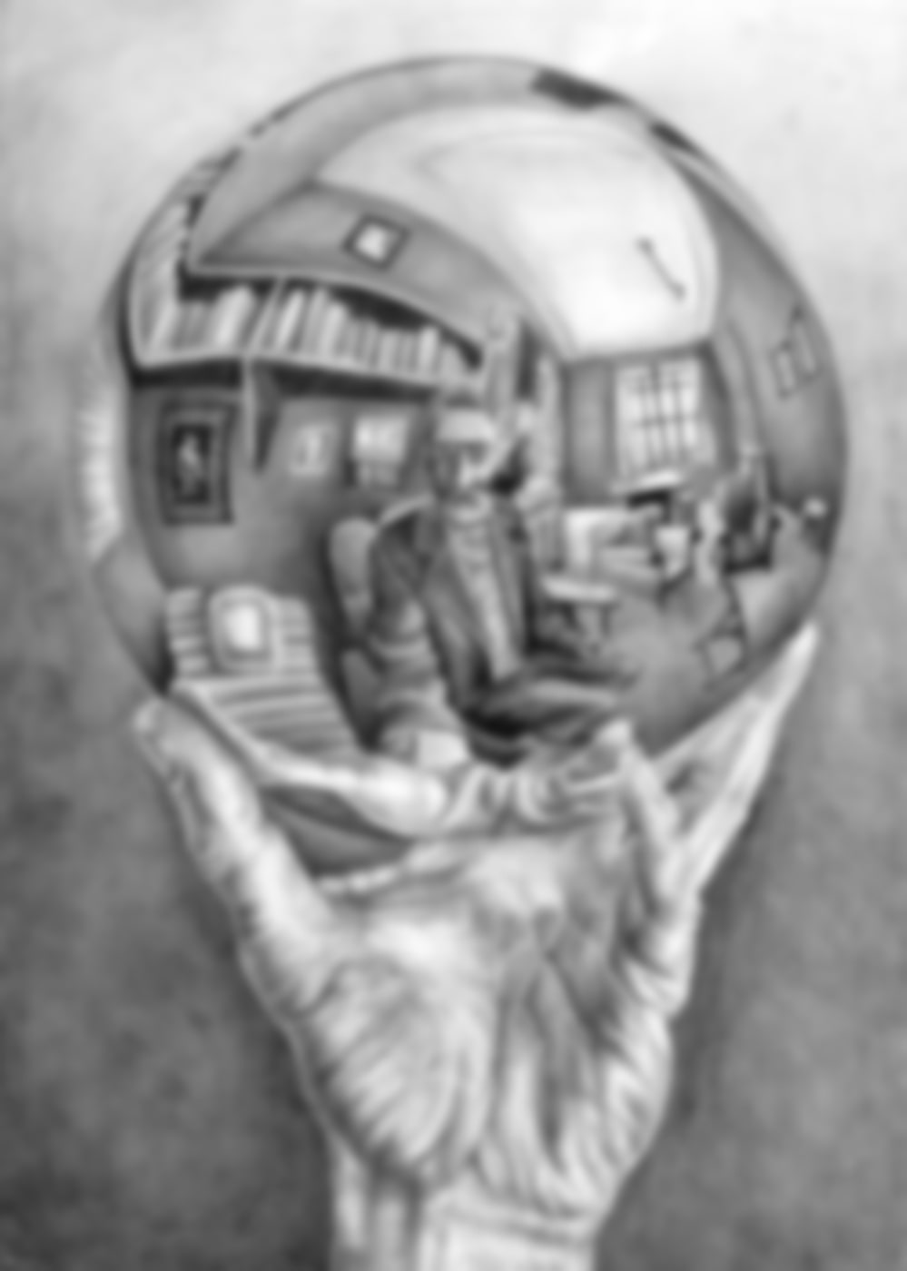


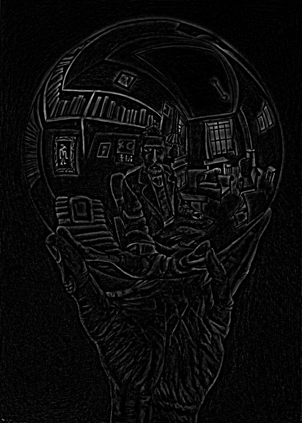
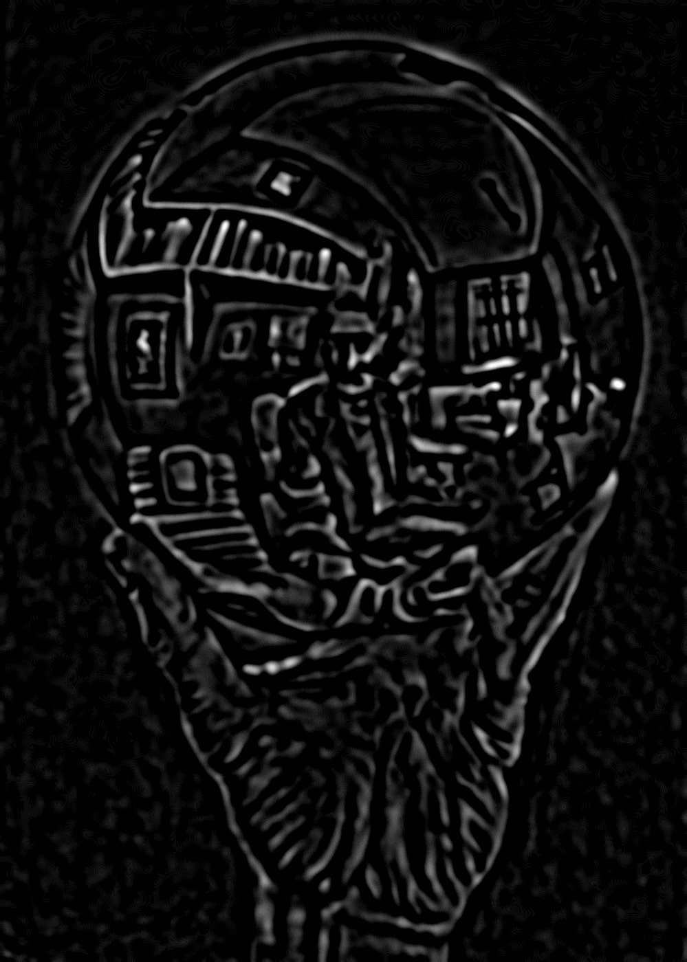

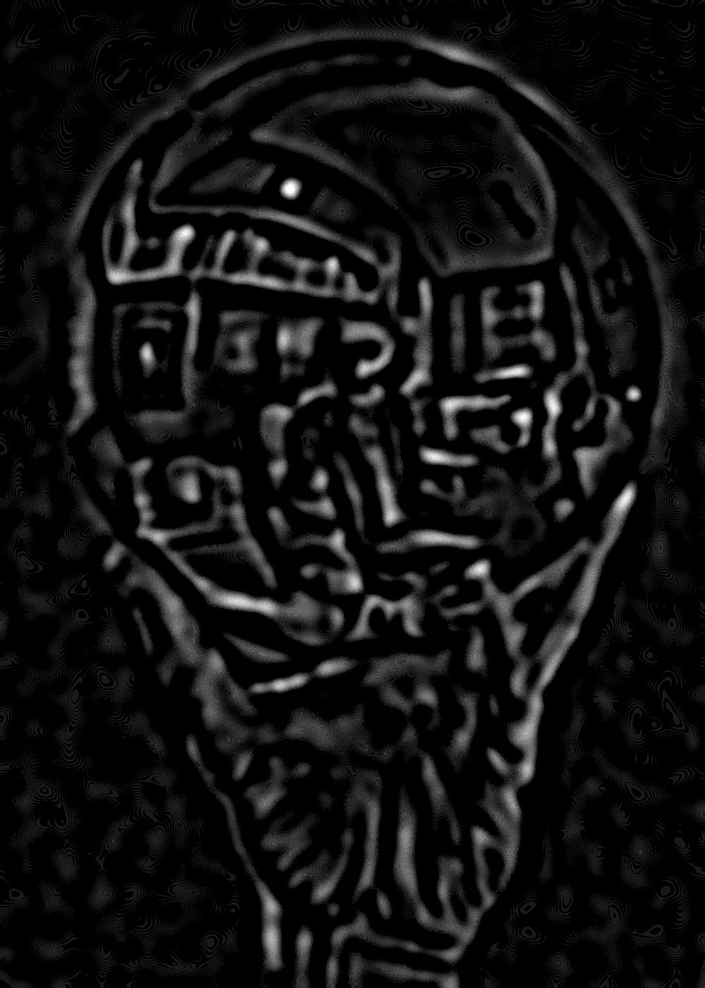
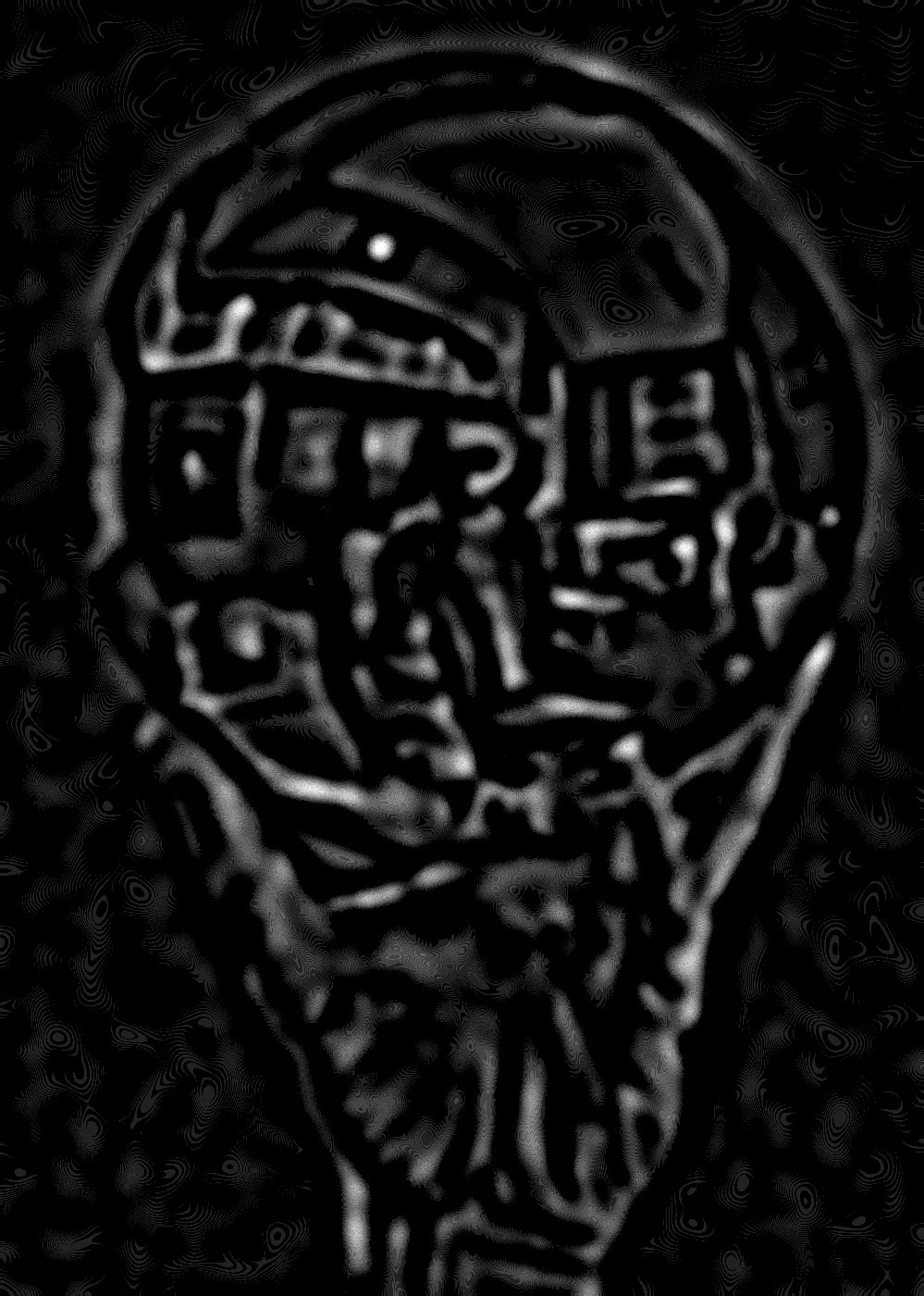
Different structures come to light at different levels in the stack for surrealist artist M. C. Escher’s Hand with Reflecting Sphere.


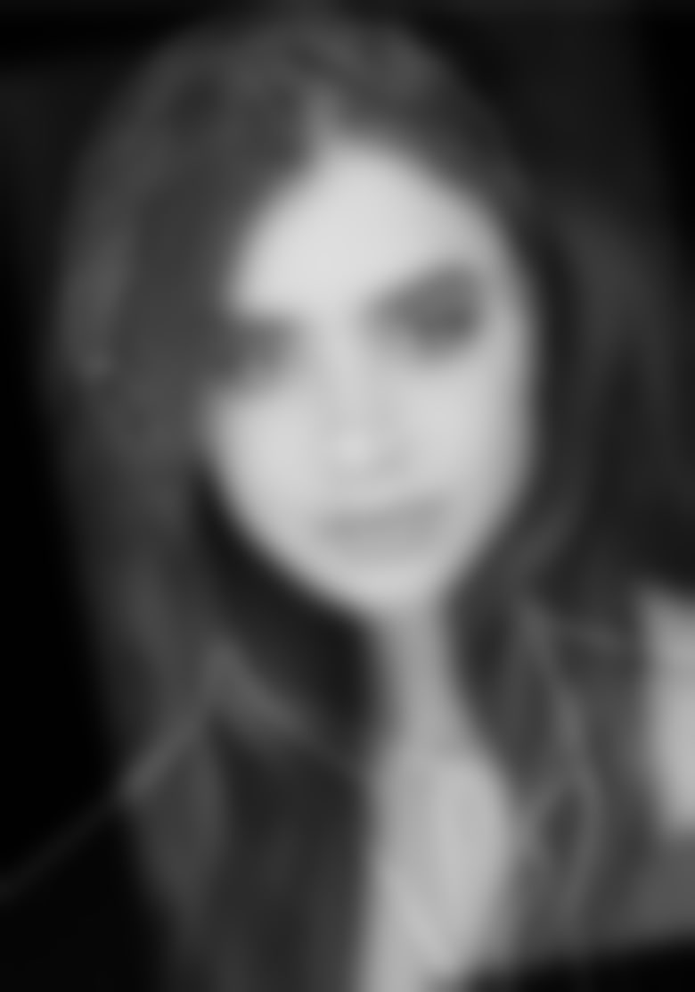
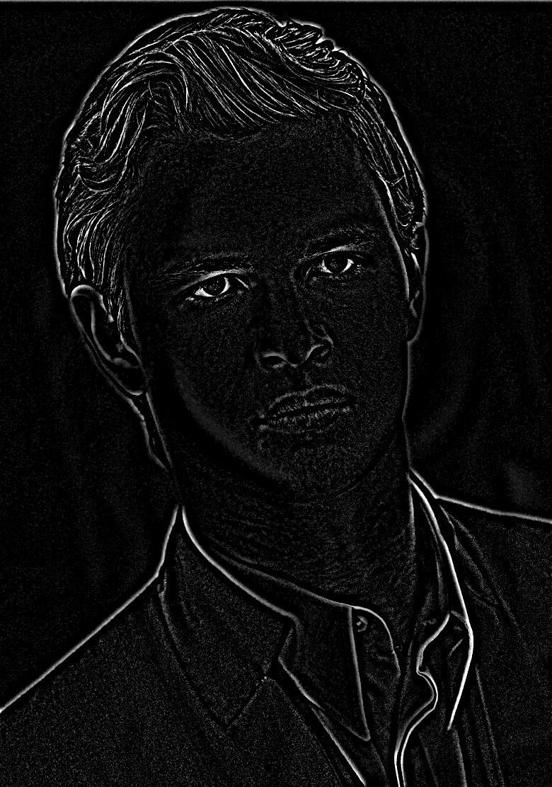
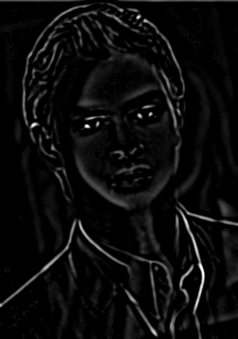
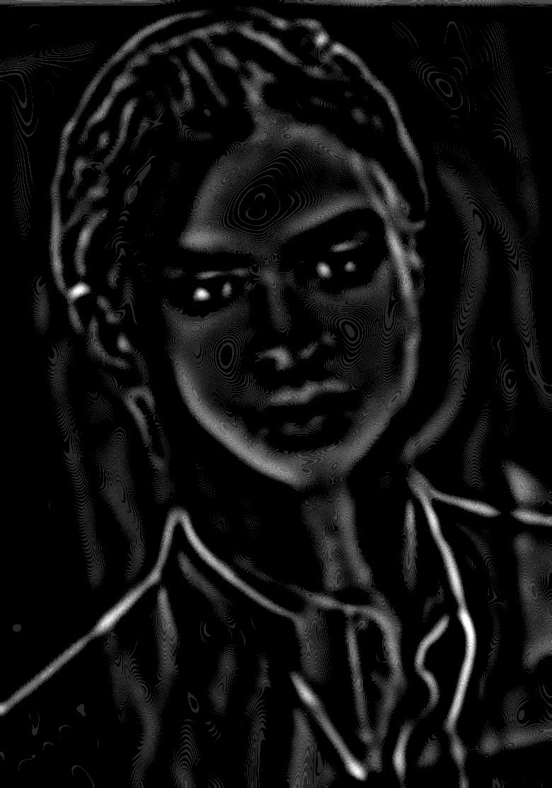
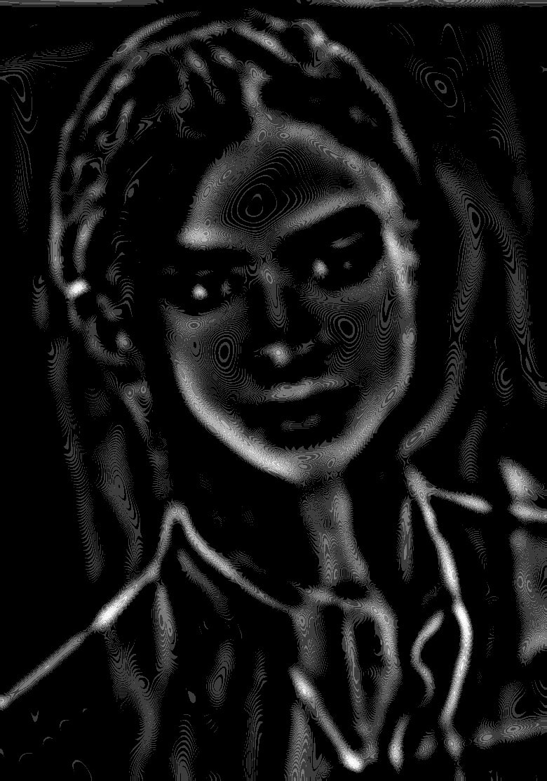
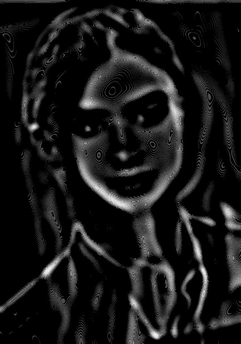
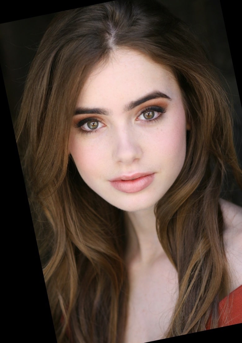
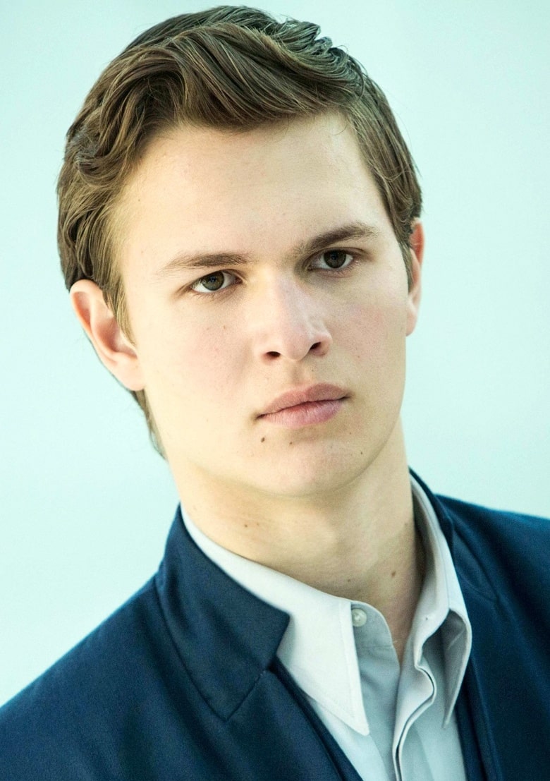
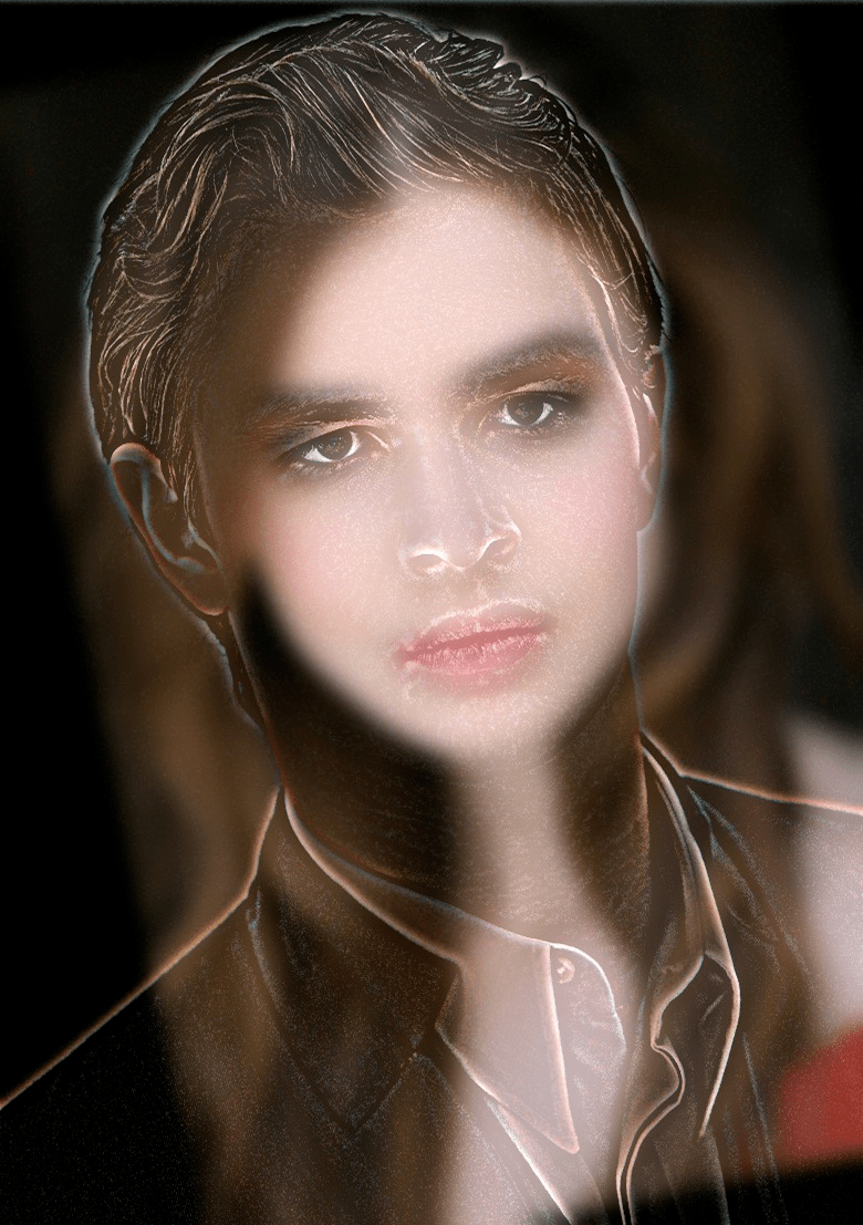
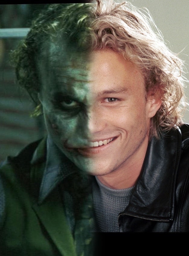
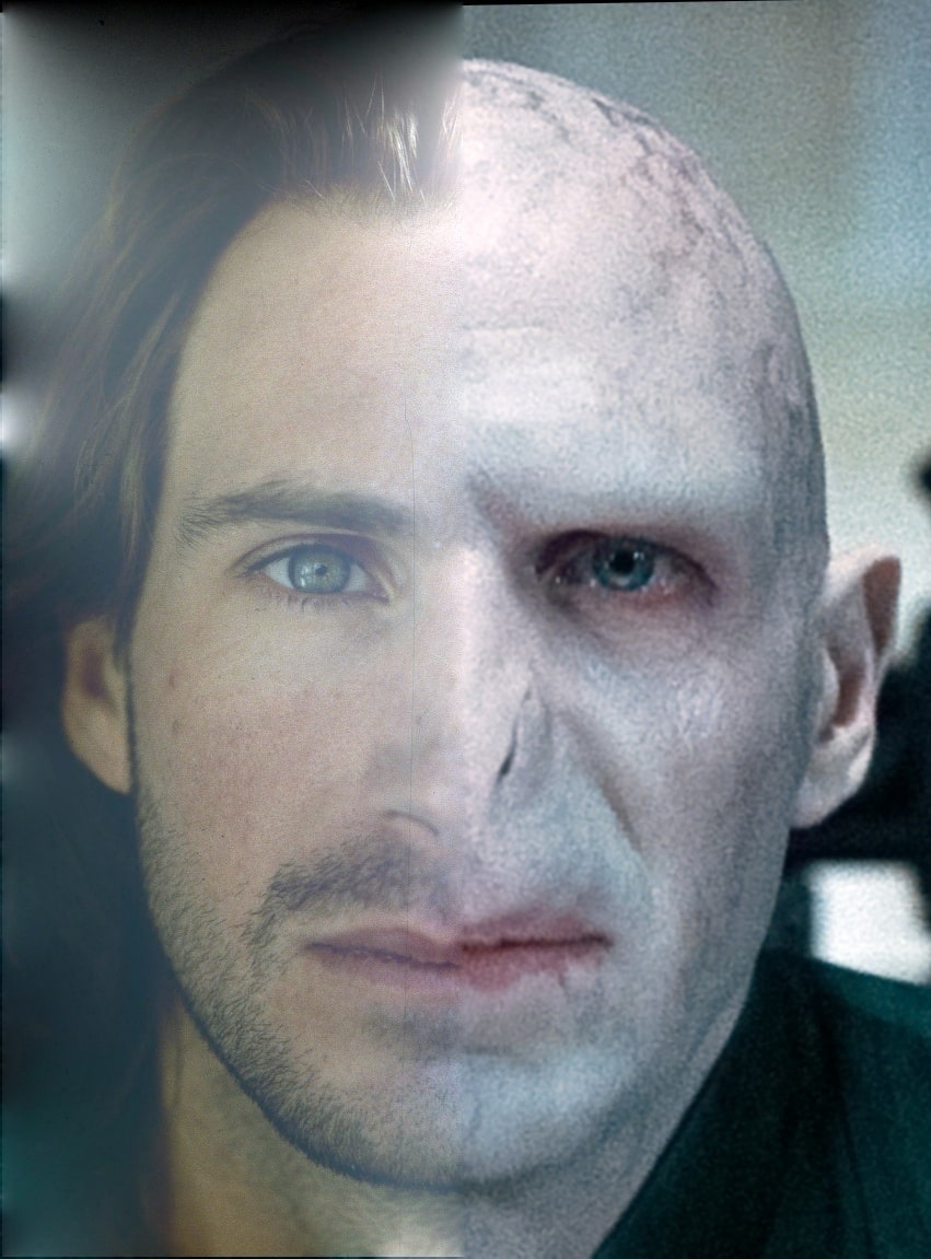
Looking at the stacks for the hybrid image we created earlier reveals the transition from high-frequency Ansel Elgort to low-frequency Lily Collins, as expected.
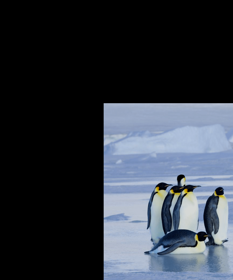
Part 1.4: Multiresolution Blending
An image spline is a smooth seam joining two image together by gently distorting them. Multiresolution blending computes a gentle seam between the two images seperately at each band of image frequencies, resulting in a much smoother seam.
We use a slight modification of the algorithm presented in the 1983 paper by Burt and Adelson. At a high-level, the steps are as follows:
- For input images A and B (of the same size), build Laplacian stacks \( LA \) and \( LA \).
- Create a binary-valued mask M representing the desired blending region.
- Build a Gaussian stack \( GM \) for M.
- Form a combined stack \( LS \) from \( LA \) and \( LB \) using values of \( GM \) as weights. That is, for each level \( \ell \),
- Obtain the splined image S by expanding and summing the levels of \( LS \).
Essentially what we’re doing is using higher feathering on low-frequency parts of the image and lower feathering on high-frequency parts of the image.
Some results using vertical masks are shown below:
We can also irregular masks to produce results like the following:

Below we illustrate the process by displaying the Laplacian stacks for both input images (shown with the mask already applied).

Part 2.1: Toy Problem
To warmup with gradients, our task is to reconstruct an image given a single pixel value from the original image as well as the gradient of the original image. We can accomplish this setting up a system of linear equations, \(Ax = b\). The \(x\) vector, with dimensions (height * width, 1), represents the vectorized version of the pixel values we want to reconstruct. \( A \) is a sparse matrix with dimensions (2 * height * width + 1, height * width); the first height * width rows in \( A \) correspond to the x-gradients for each pixel and the next height * width rows in \( A \) correspond to the y-gradients of each pixel. The last row ensures that the top left corners of the two images are the same color. The \( b \) vector, with dimensions (2 * height * width + 1, 1), contains the corresponding results to the gradient equations in the \( A \) matrix.
Using a least squares solver, we get the correct reconstruction result. The original image is shown on the left and the reconstructed image is shown on the right.


Part 2.2: Poisson Blending
Background
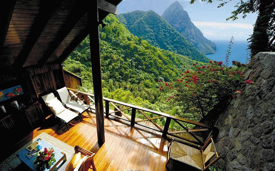
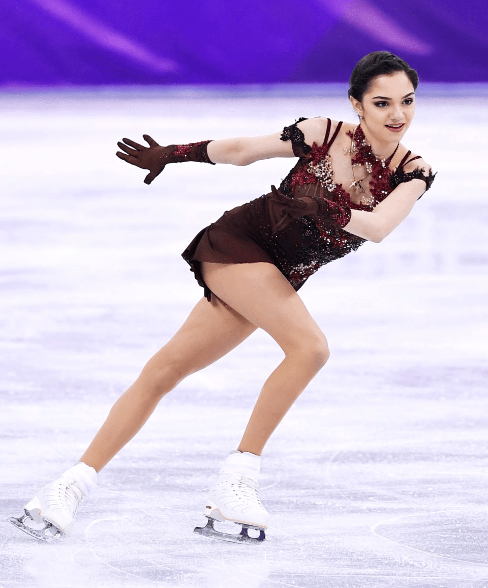
We'll now look at an application of gradient-domain processing known as Poisson blending. The goal is to seamlessly blend an object or texture from a source image into a target image. Unlike our previous approach, we'll work with the gradient of the image; the task is finding values for the target pixels that maximally preserve the gradient of the source region without changing any of the background pixels. It can be formulated as a least squares problem.
Given the pixel intensities of the source image \( s \) and of the target image \( t \), we want to solve for new intensity values \( v \) within the source region \( S \) (as specified by a mask):
Here, each \( i \) is a pixel in the source region \( S \) and each \( j \) is a 4-neighbor of \( i \) (left, right, up, and down). The first term expresses that we want an image whose gradients inside the region \( S \) are similar to the gradients of the cutout we’re trying to paste in. The least squares solver will take any hard edges of the cutout at the boundary and smooth them by spreading the error over the gradients inside \( S \). The second term handles the boundary of \( S \); we just pluck the intensity value right out of the target image.
Results
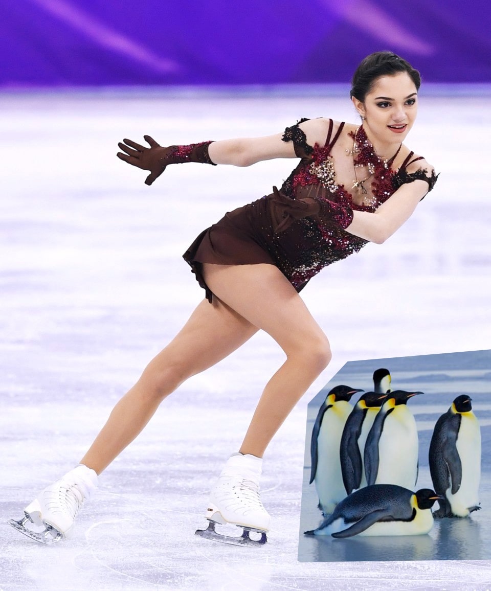
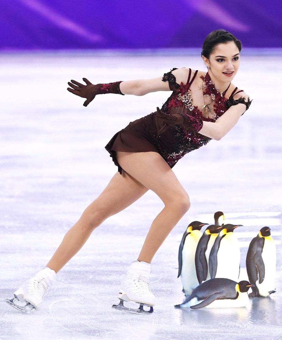
Below we show the source image, mask, and target image (top row) as well as the result of directly copying source pixels onto the target region, and finally the result of Poisson blending (bottom row) for a few successful cases.

A few more decent results are shown below:
We now show a failure case:
What went wrong here? The problem is that the gradient of the target region is very rough while the gradient of the source region is smooth. The inevitable error from trying to match the gradients is spread across the source image, and the intensity values are noticeably off as a result.
We can also compare the results of Poisson blending with multiresolution blending. Shown below are the results of multiresolution blending (left) and Poisson blending (right).
The choice of appropriate blending method depends on the desired result. Multiresolution blending is ideal when the colors and intensities of the source and target should be preserved. It is also much faster than Poisson blending. However, Poisson blending is great for the case in which the target and source regions have similar textures and we wish to seamlessly clone the source onto the target without a noticeable change in intensity.
Reflection
This project was a lot of fun. Nothing was particularly difficult, but it was very time-consuming as a whole. The most important thing I learned was to constantly experiment and interact with the code by visualizing the results. Nothing in this field is an exact science and you only learn by trying things and seeing what works (and what doesn't). On a practical level, I learned more about OpenCV and how to vectorize code with numpy.