Project Spec: https://inst.eecs.berkeley.edu/~cs194-26/fa18/hw/proj3/index.html

Part 1: Frequency Domain

Part 1.1 Image Sharpening

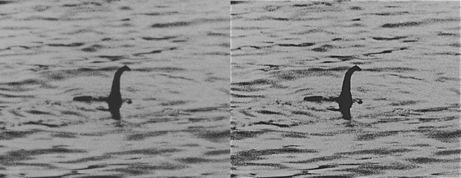
Let's begin by examining some blurry photos of purported creatures.

Here's Nessie, swimming in his (or her) home in Loch Ness. Sharpening the image does very little since it's blurry with few visually interesting details.

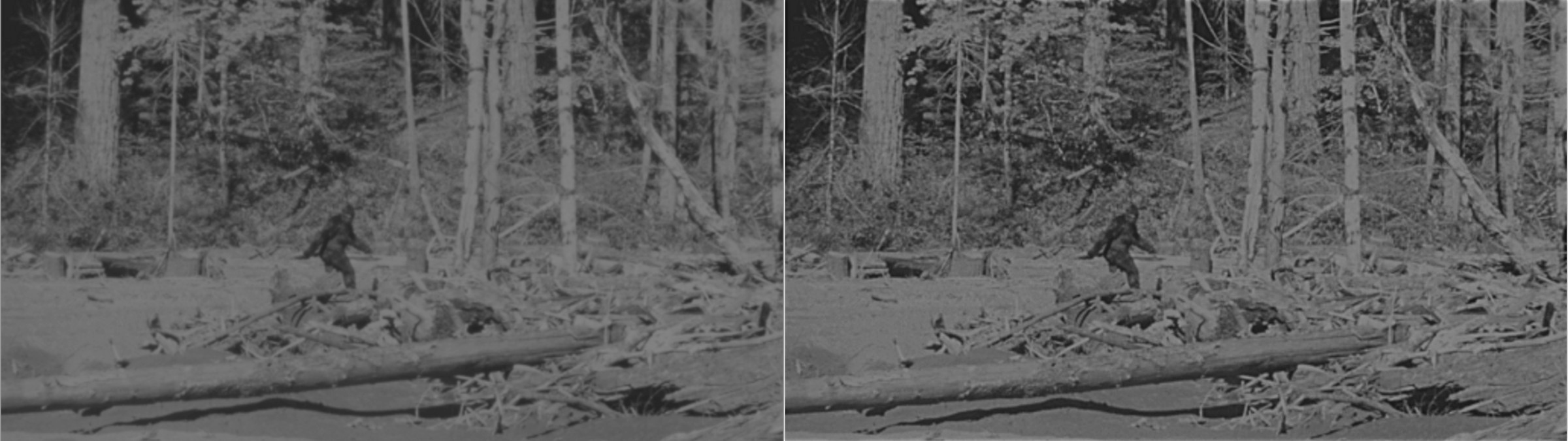
Bigfoot, on the other hand, sees a significant improvement after applying such a basic sharpening technique.

Part 1.2 Hybrid Images

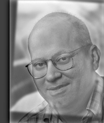
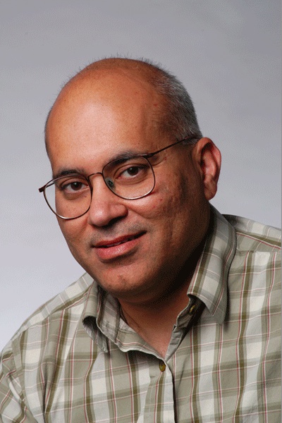
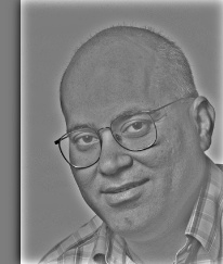
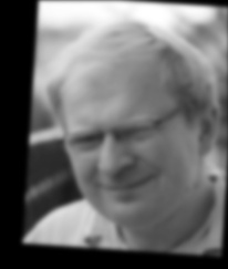
Now, I present esteemed computer vision professor Altendra Efrolik:

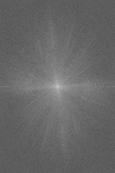
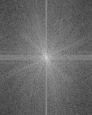
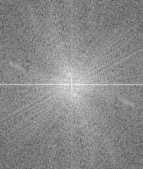
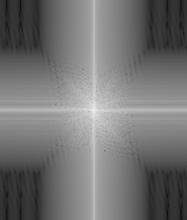
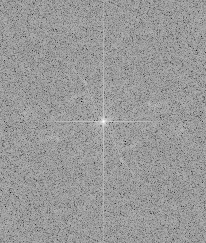
We can also perform a frequency analysis by visualizing the log Fourier transforms.

Here are the input images:

High pass image:

Low pass image:

Hybrid image:

Some more hybrid results

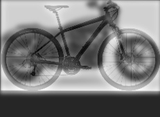
Motorbike (motorcycle + bike)

Pandar (panda + polar bear). This one did not work well because they aren't properly aligned.

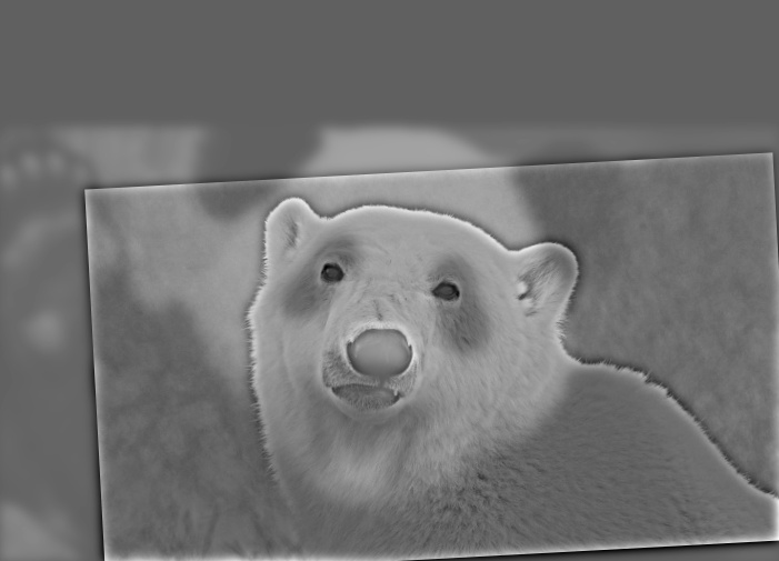Part 1.3 Gaussian and Laplacian Stacks

Gaussian and Laplacian stacks provide a convenient way to visualize the different frequency bands for an image.

Here is Salvador Dali's Gala Contemplating the Mediterranean Sea which at Twenty Meters Becomes the Portrait of Abraham Lincoln:

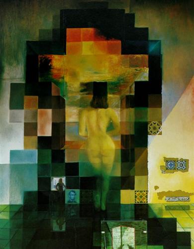The high frequencies (viewed up close) show Gala while the lower frequencies (viewed from a distance) show Abraham Lincoln.

The Gaussian stack can be used to visualize the lower frequencies.

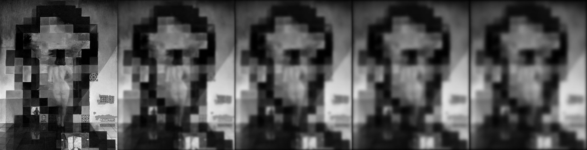The Laplacian stack shows the different bands of frequencies.

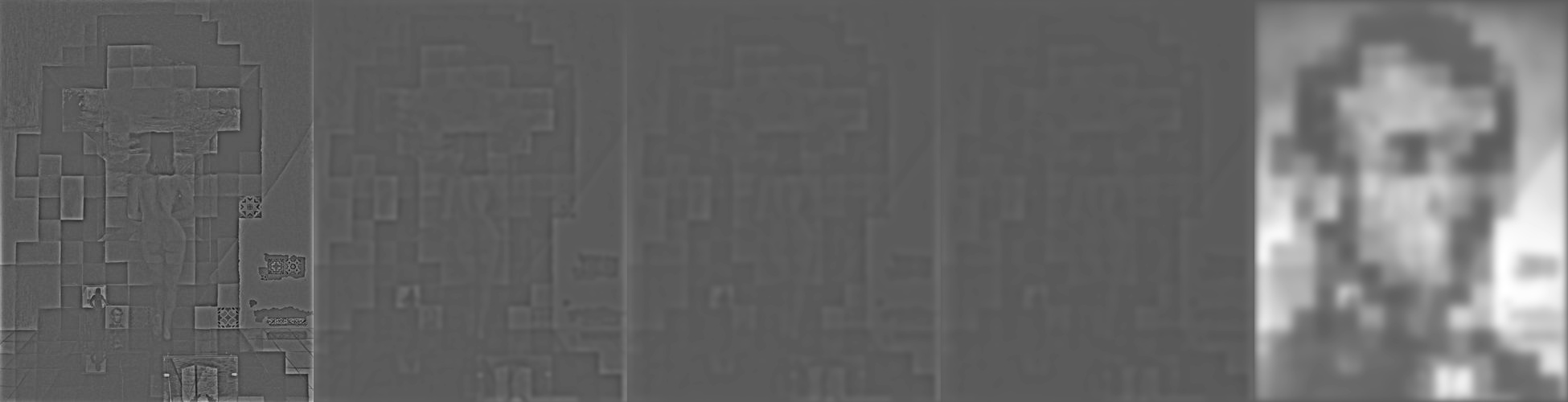Here is Leonardo da Vinci's Mona Lisa:

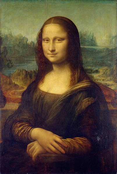The high frequencies (viewed with central vision) make her appear to be frowning while the low frequencies (viewed with peripheral vision) make her appear to be smiling.

The Gaussian stack can be used to visualize the lower frequencies.

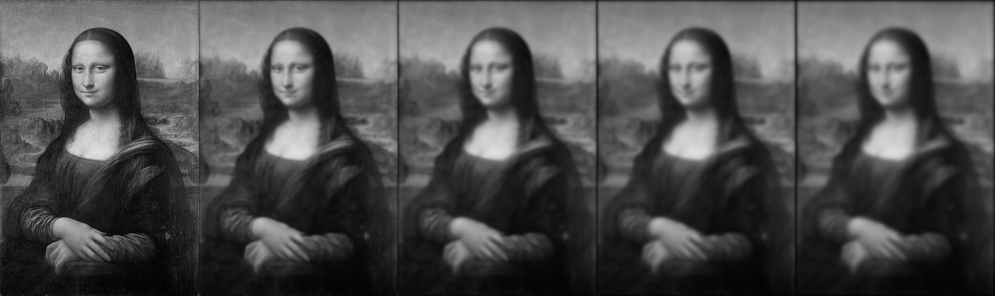The Laplacian stack shows the different bands of frequencies.

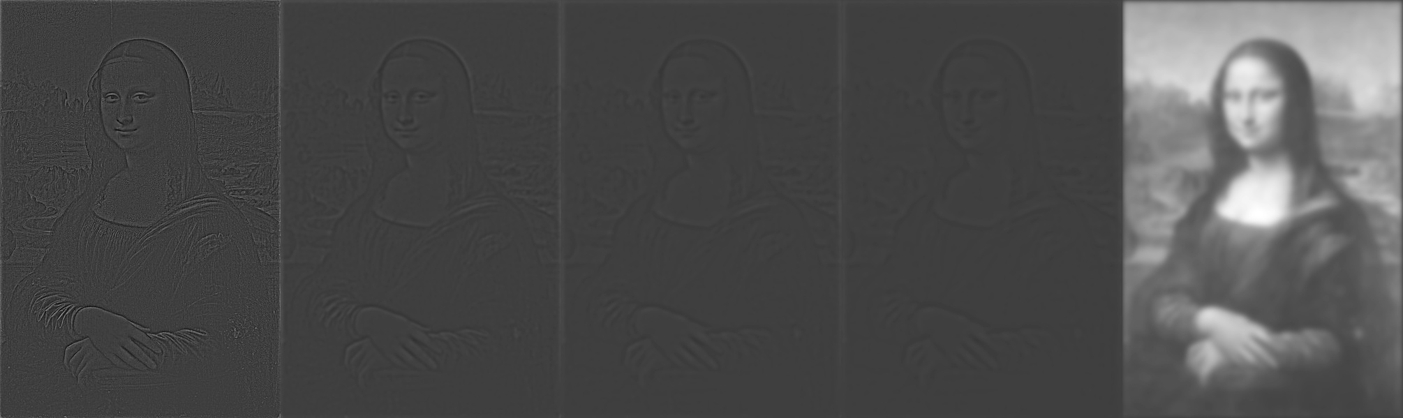We can also visualize Professor Efrolik at different frequencies.

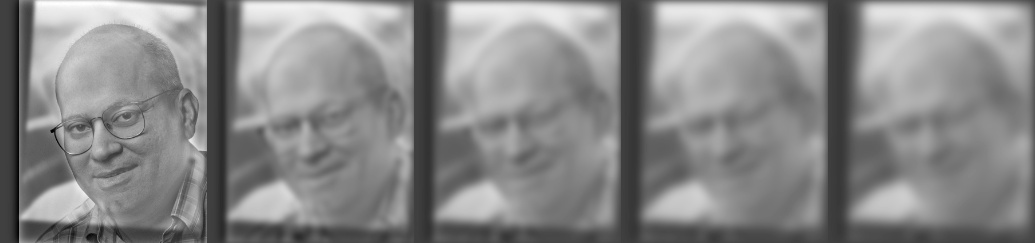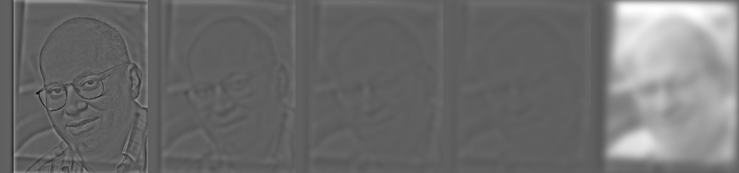Part 1.4 Multiresolution Blending

We can seamlessly blend together two images by feathering two images at different frequencies using the bands of the Laplacian stack.

For example, we can blend together an apple or orange

thus forming the applange and orapple!

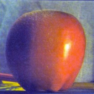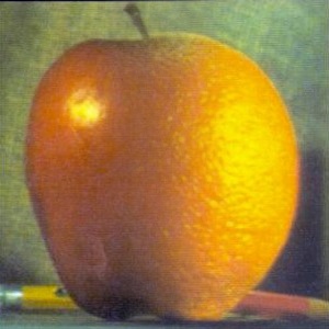Here is the most feared bounty hunter in the galaxy!

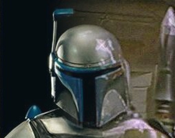We can also make Trumpkin!

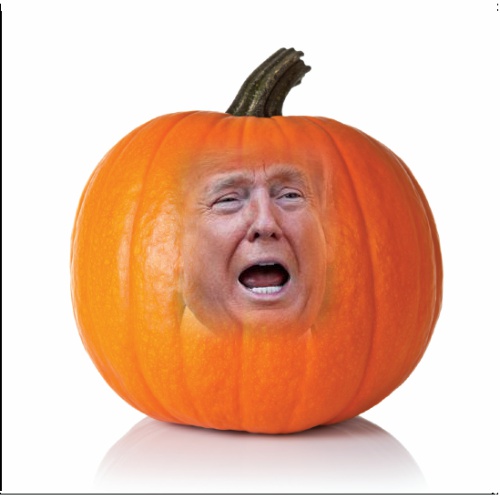Part 2: Gradient Domain Fusion

Part 2.1: Toy Problem

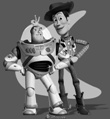
I began by recreating Buzz and Woody by solving the optimization problem that minimizes the difference between the x-gradients and y-gradients between the source and target image with the additional constraint that the top left corners must be the same color.

Using a least squares solver, I can find the set of pixel values that minimizes the objective equations, which reproduces the original image.

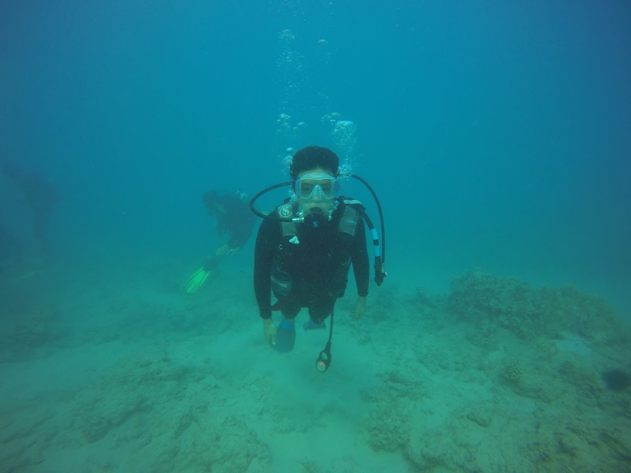
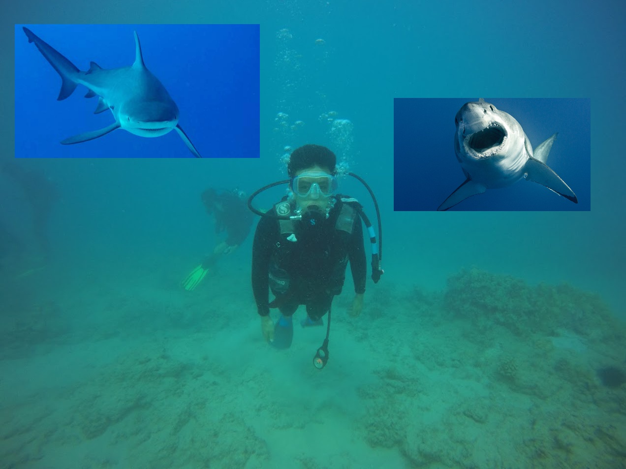
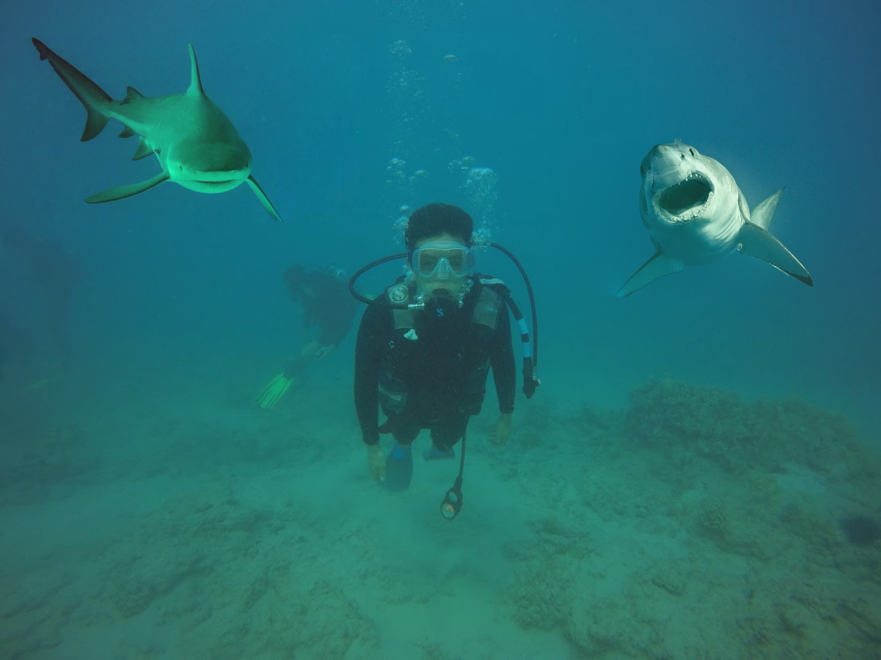
Part 2.2: Poisson Blending

Now we can do more interesting things through Poisson blending. The goal is to more seamlessly embed a source image into a target image by working in the gradient domain. Here, the objective function is to preserve the gradients of the original image (first half of the objective) while also preserving the gradients along the edges of the target image (second half).

Original images:

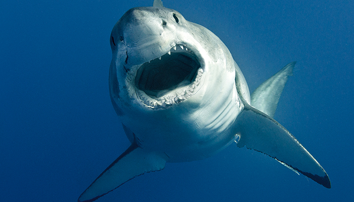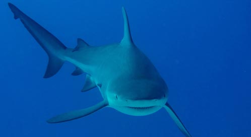The left shark's original image was already too blue.

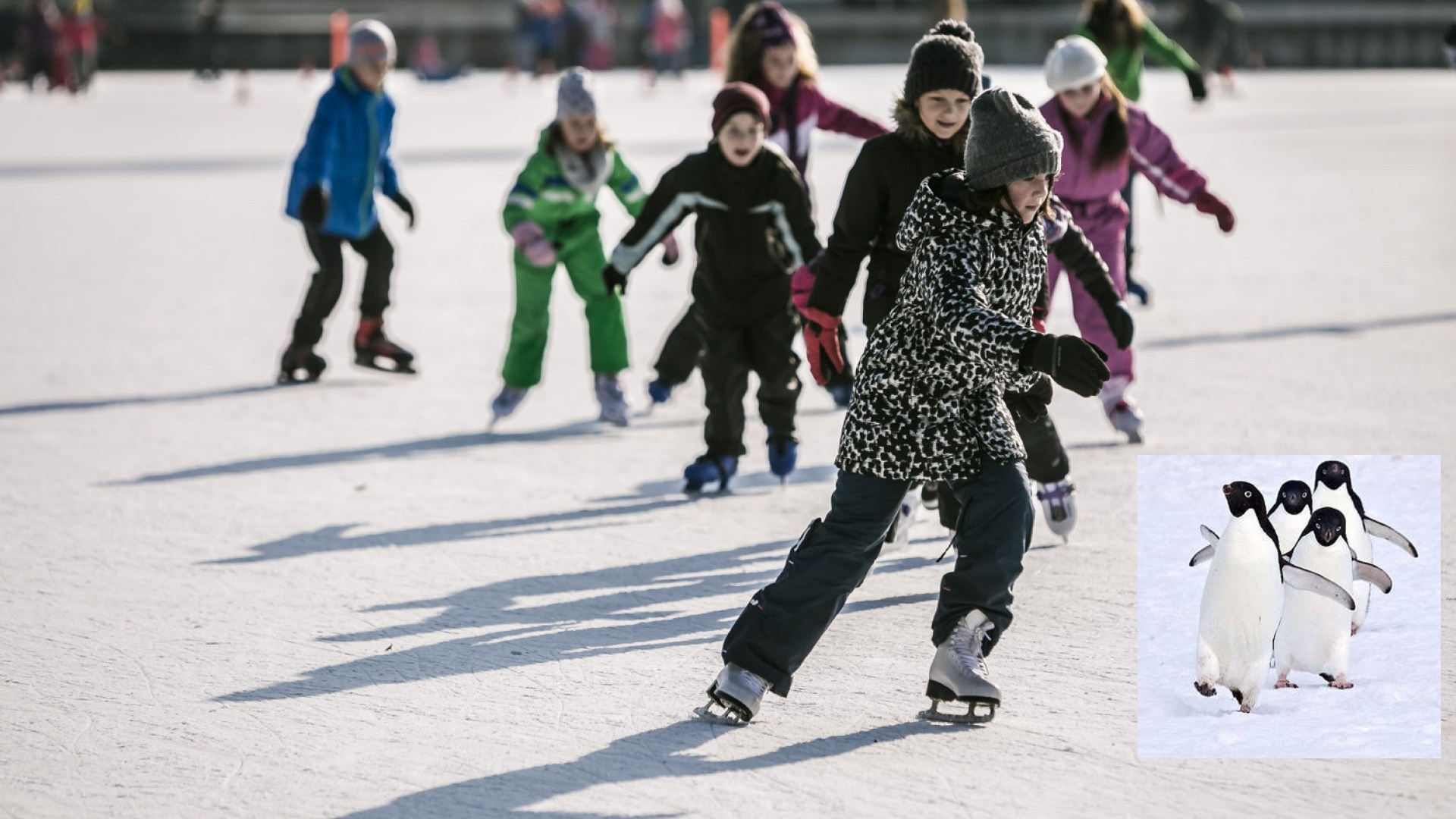
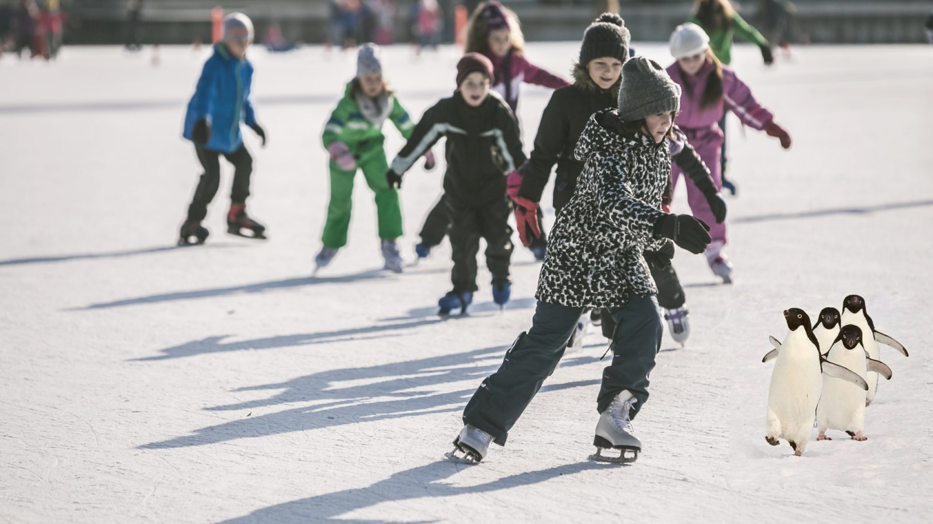
Skating with penguins. Notice that the lighting of the penguin doesn't match that of the skaters, and the shadows are completely off.

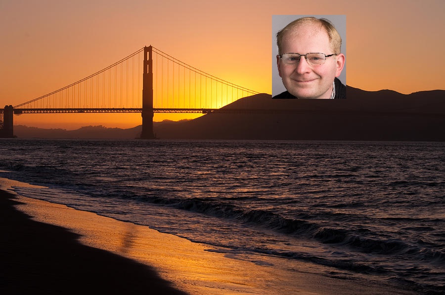
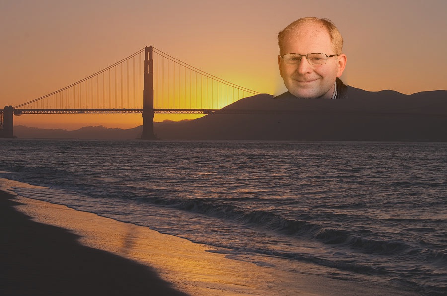
The most beautiful sunset I've ever seen.

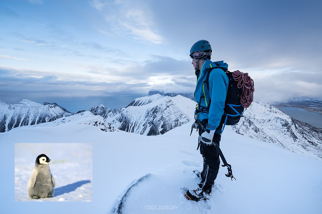
Here's an obvious failure due to the texture of the penguin's snow.

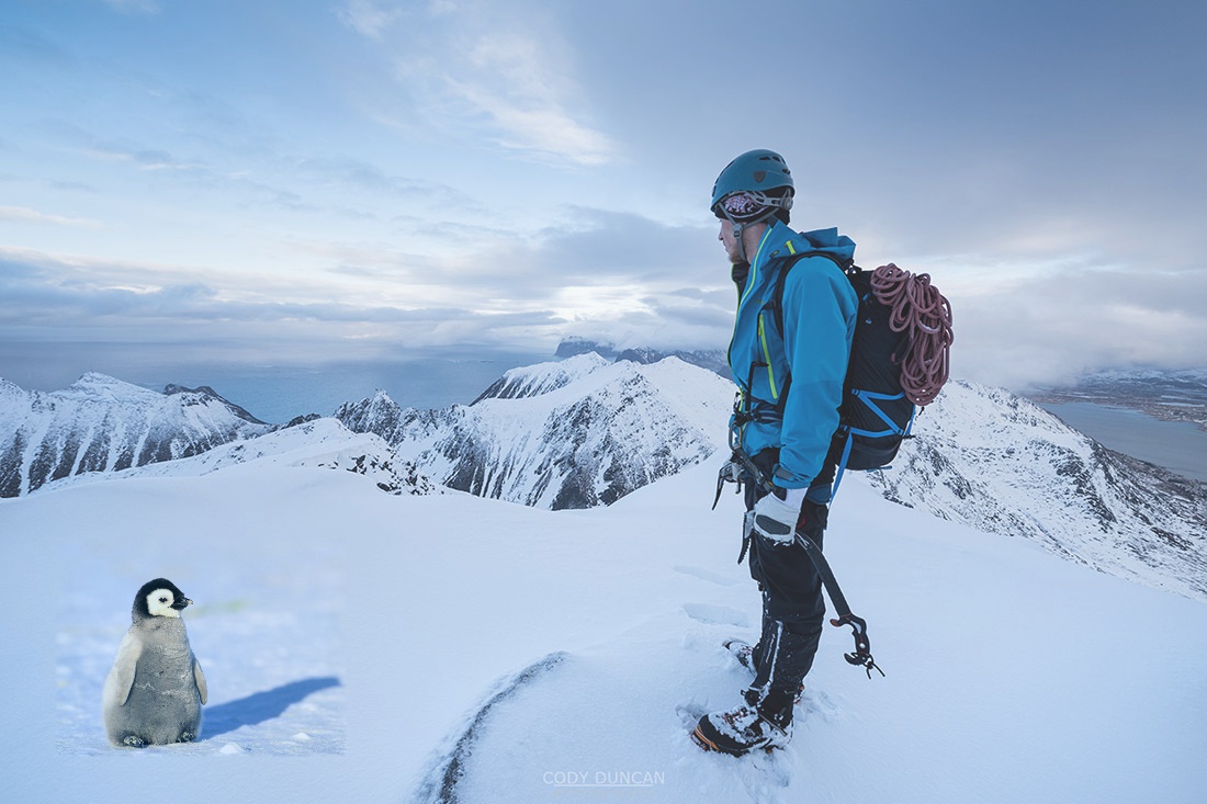Here we compare blending using Multiresolution blending and Poisson blending. I think Poisson blending looks better since the orange color really suits Donald.
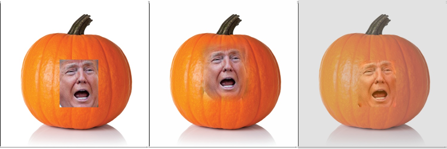