Overview
In this project, we investigate different techniques for performing image blending. Part 1 of the project uses frequency domain analysis to sharpen blurry images, create hybrid images, and do seamless multiresolution blending. Part 2 of the project makes use of the gradient domain of images - a domain that represents images in terms of their horizontal and vertical derivatives. Because human visual perception places more importance on high frequencies of an image - ones that are captured well by gradients - we can perform almost flawless visual blending using the gradient domain.
Part 1: Frequency Domain
Part 1.1: Warmup: Sharpening Images
Here we use the 'unsharp filter' which uses the laplacian filter to find high frequency components of the image. Then, the high frequency components are added back to the image with a weight a - when a is larger than 0, we see a boost in the high frequencies.
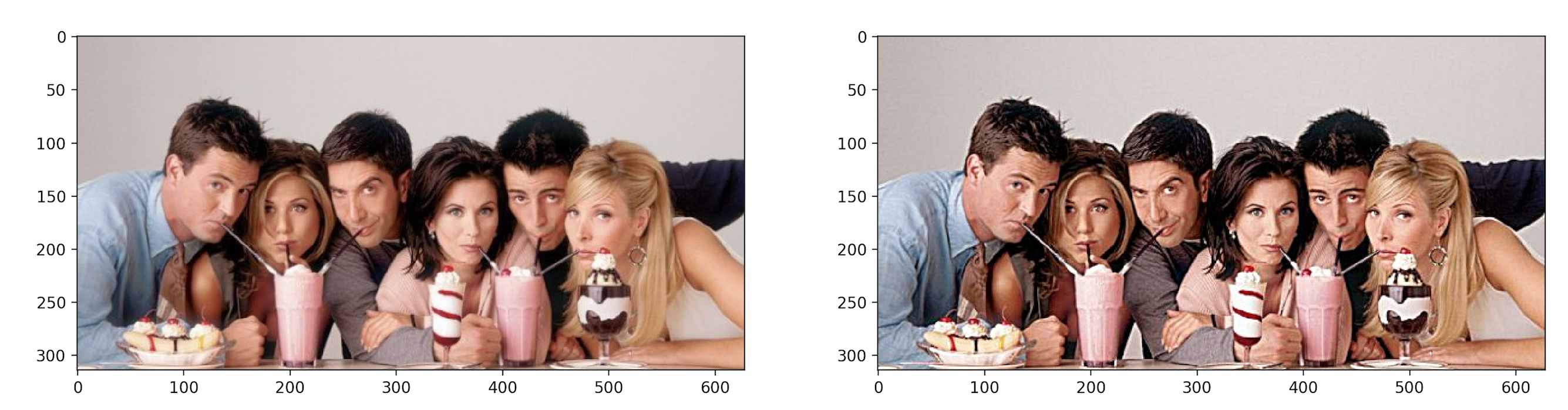 Sharpened image of the actors of my favorite tv show Friends
|
Part 1.2: Hybrid Images
Here we create hybrid images that appear as two different images, depending on the distance from which one observes them. The underlying concept behind this technique is that high frequencies dominate visual perception. When we take the high frequencies of one image and the low frequencies of a another, and composite them, we multiplex the dominant frequencies. At large distances, very high frequencies cannot be seen. While at low distances, low frequencies are not dominant.
We also need to specifically choose the cutoff frequencies of the filters that we apply to each separate image. Each pair of images has a different optimal setting because of change in visual features as well as image resolution. Here we report the sigma of the Gaussian used to to compute the low-pass filter for each image. This is inversely proportional to the cutoff frequency of the filter, because as sigma increases, we average over a larger region and lose more high frequencies.
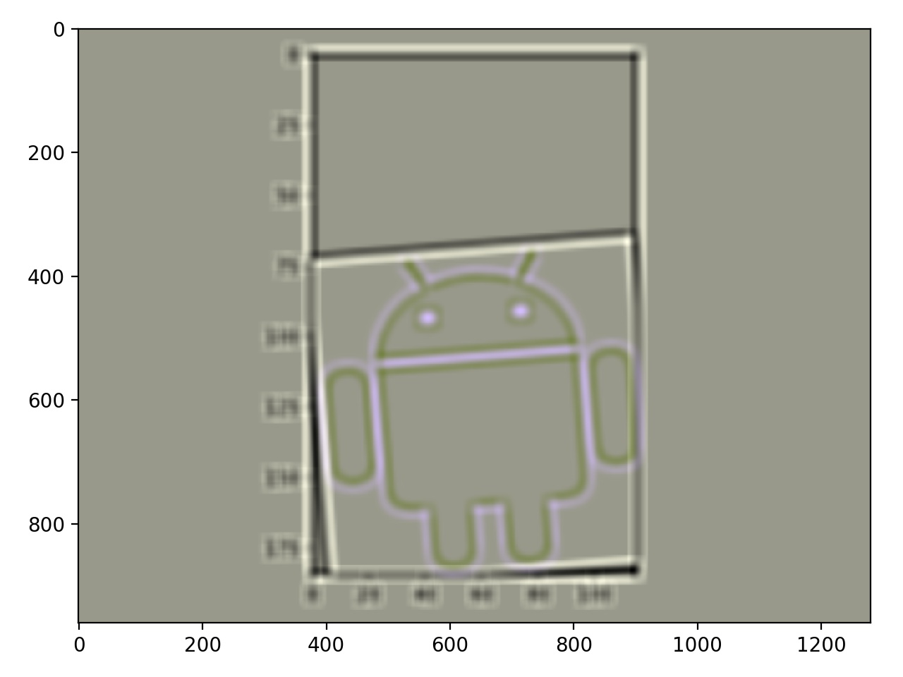
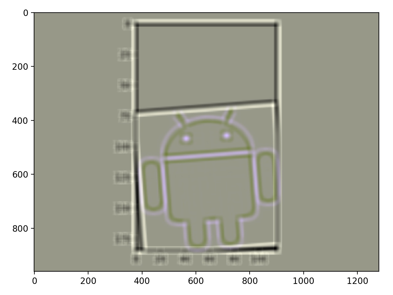
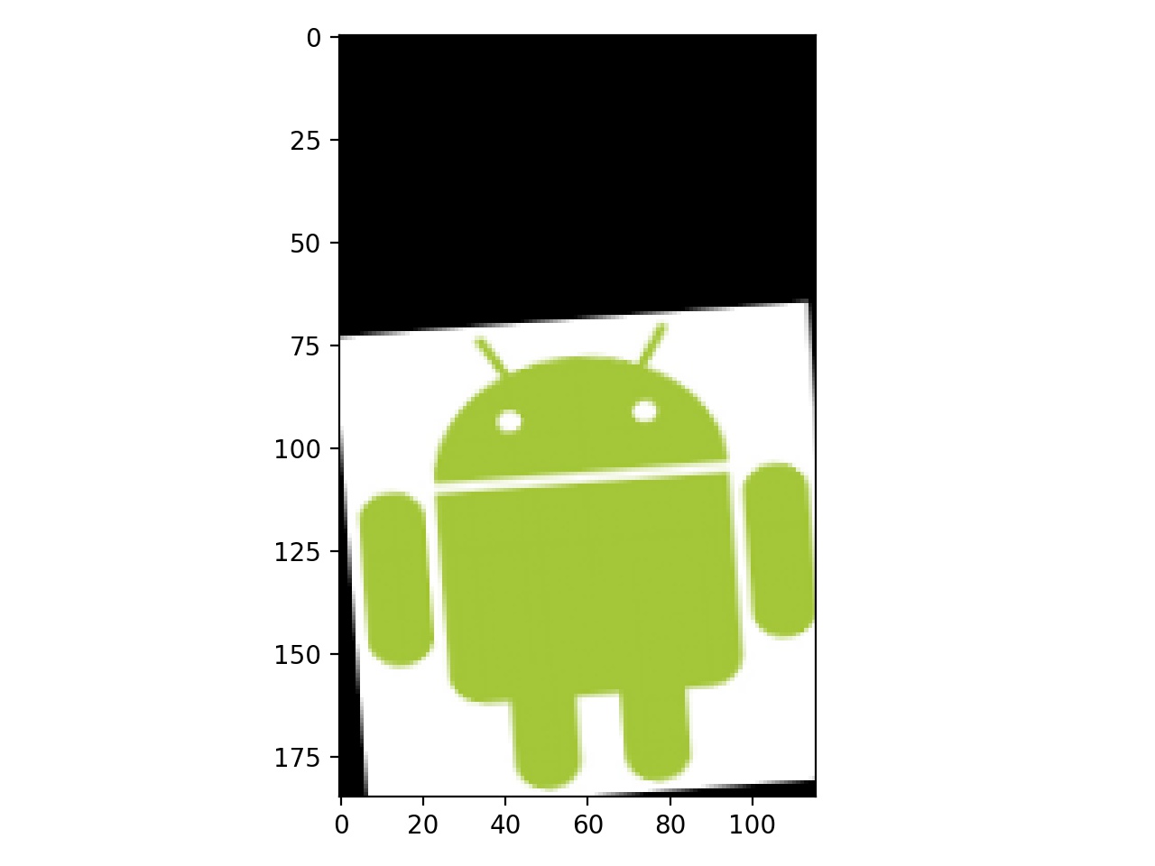 Aligned image of the Android logo
|
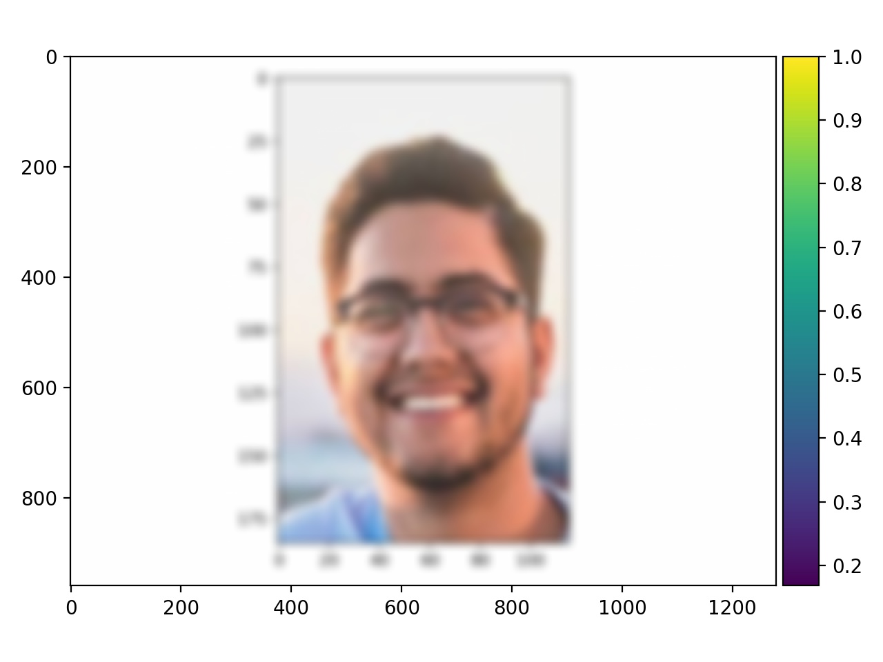
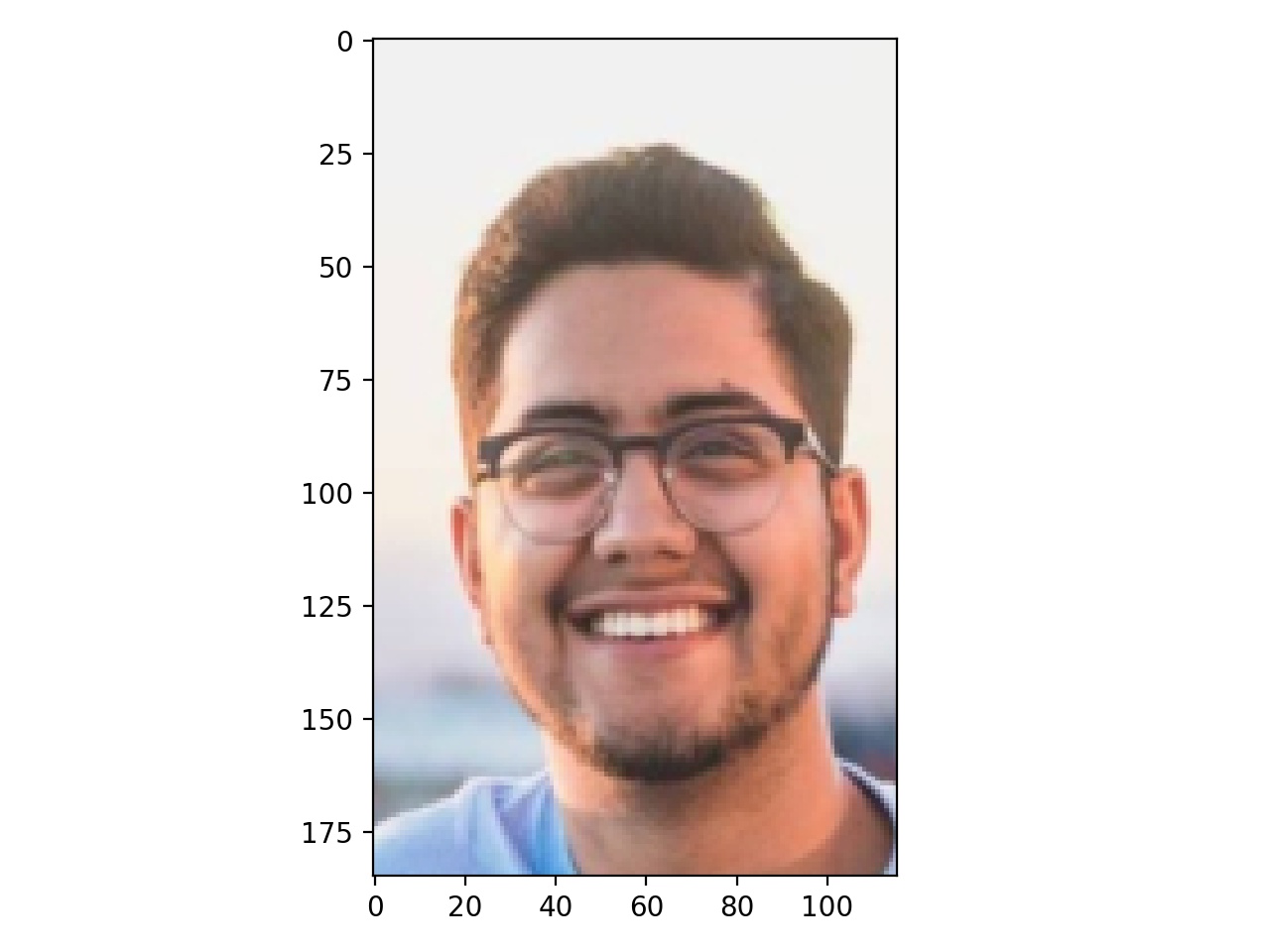 Aligned image of my face
|
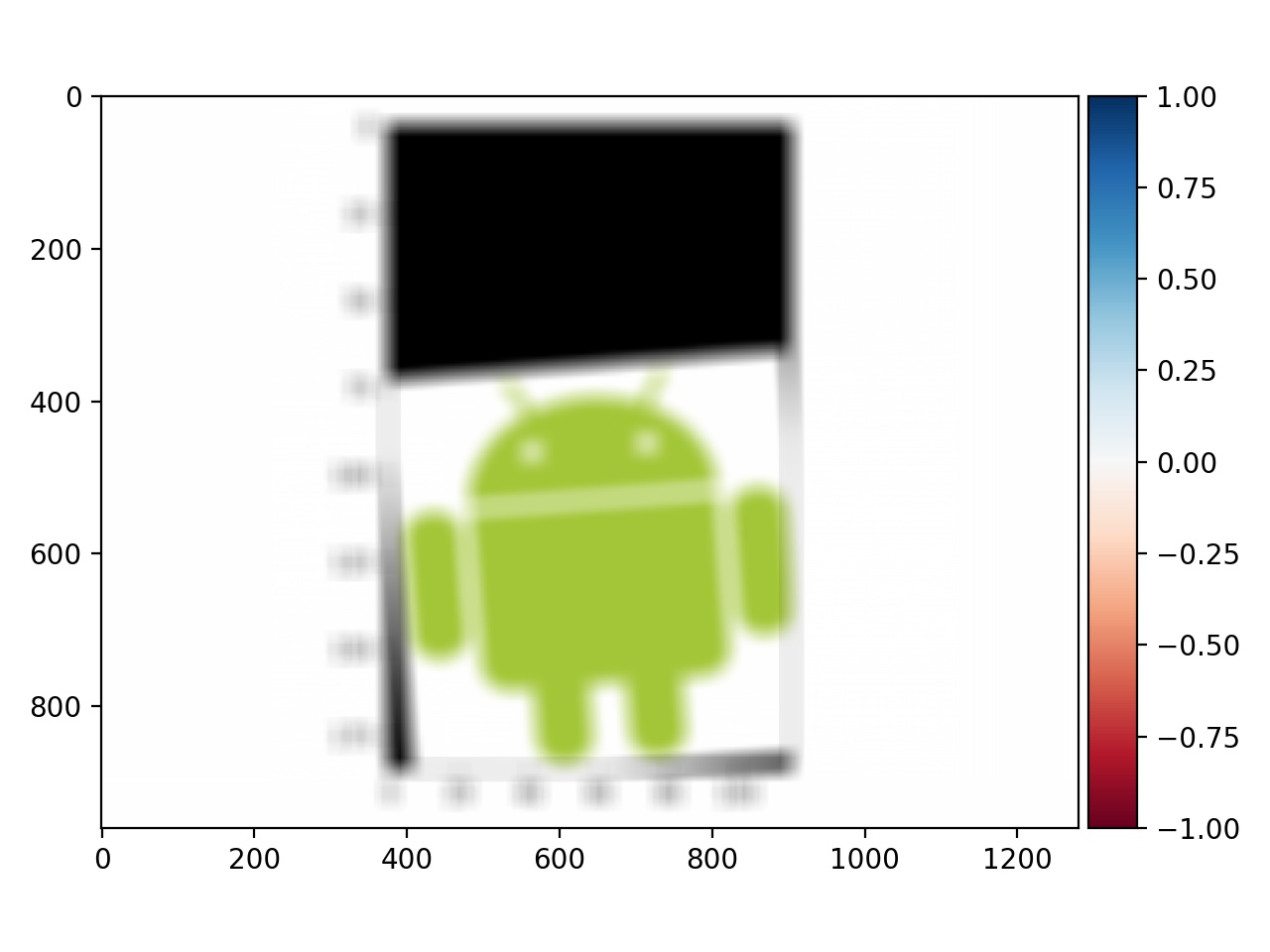
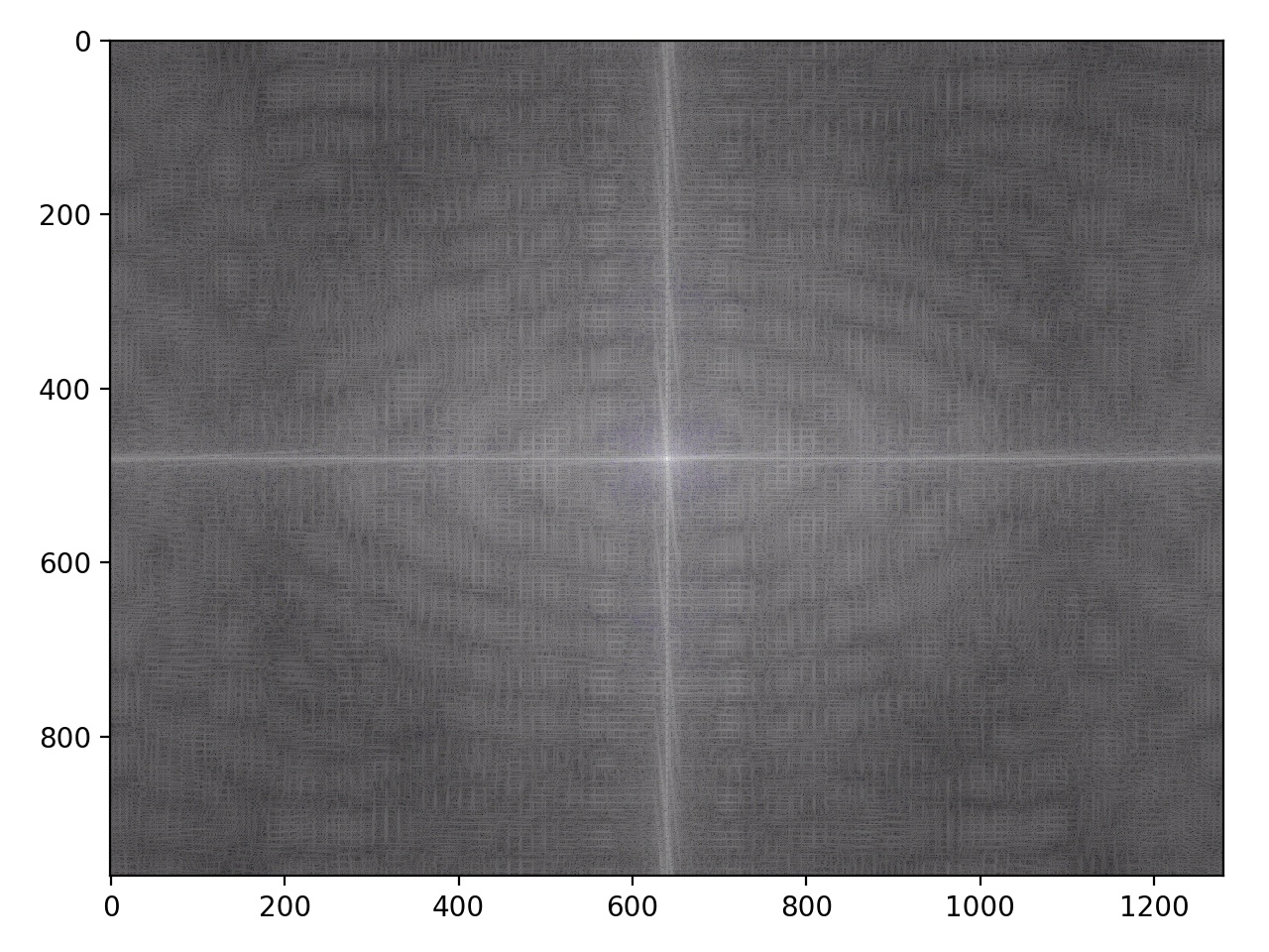 Fourier Transform of the android log
|
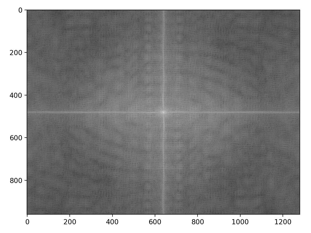
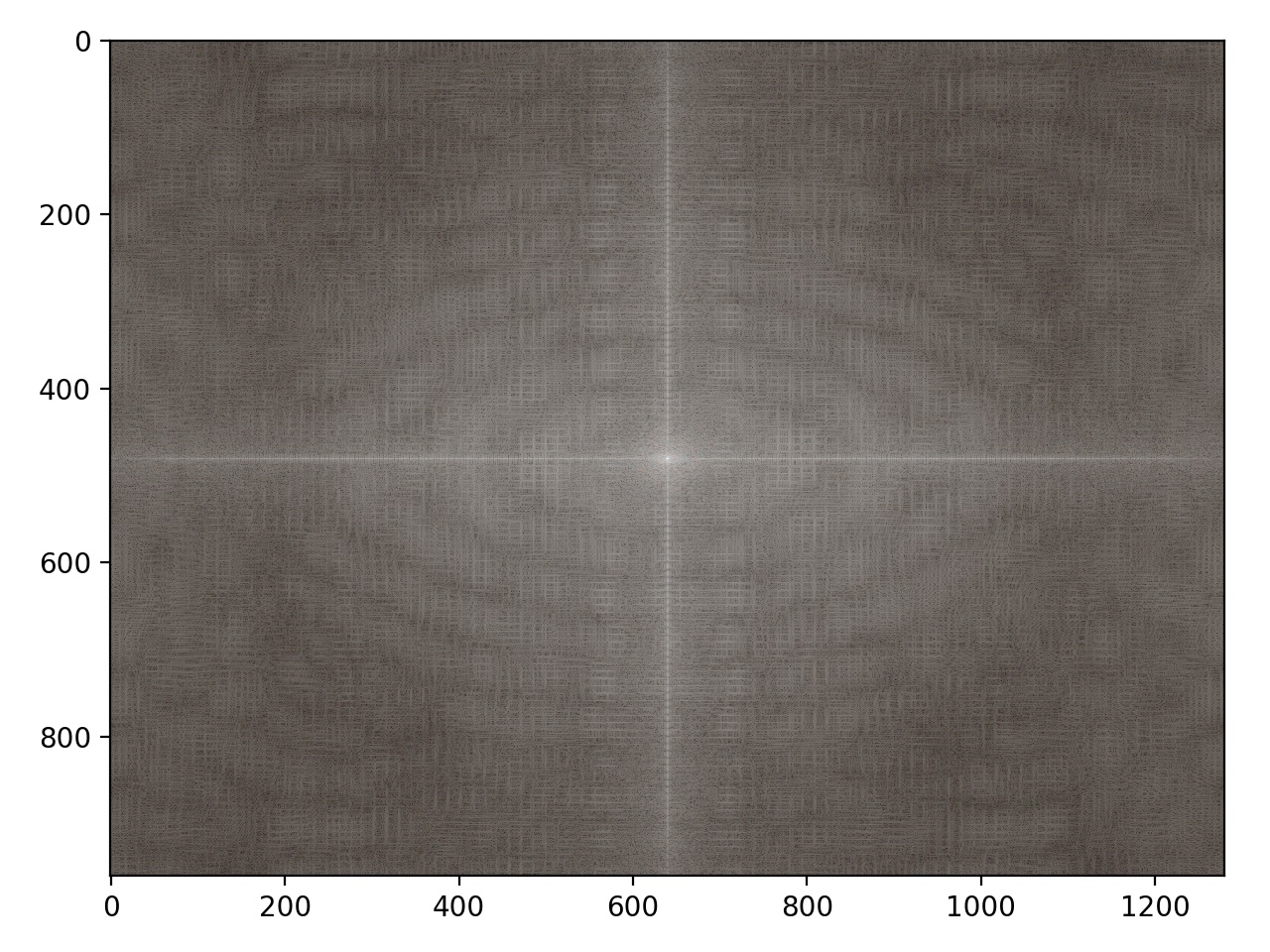 Fourier Transform of my face
|
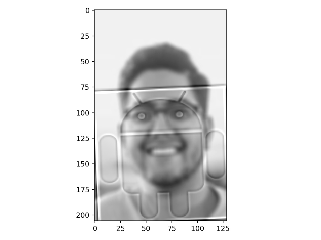 Hybrid Vivek + Android = Vivdroid
|
 Vivdroid fourier transform
|
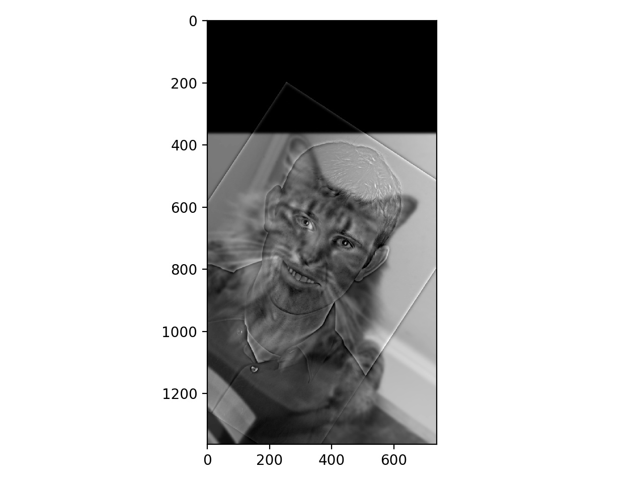 Derek + Nutmeg = dermeg
|
 Microsoft and Apple merged??
|
Part 1.3: Gaussian and Laplacian Stacks
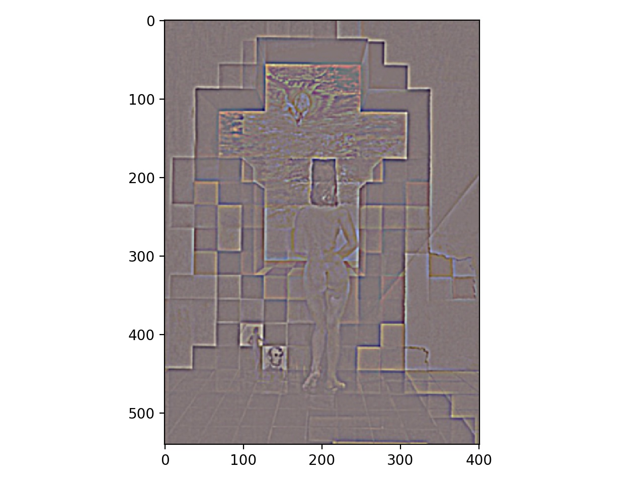
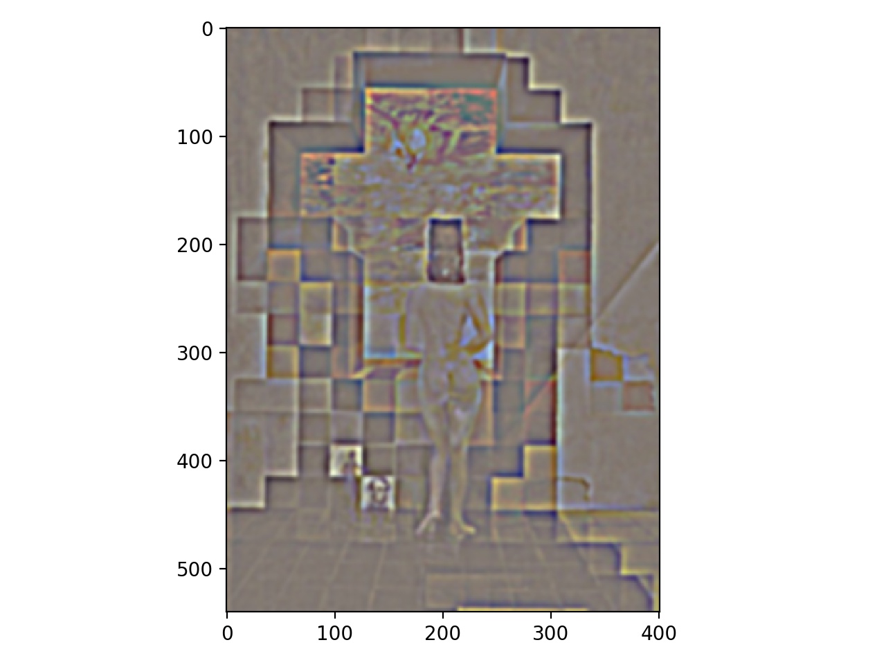
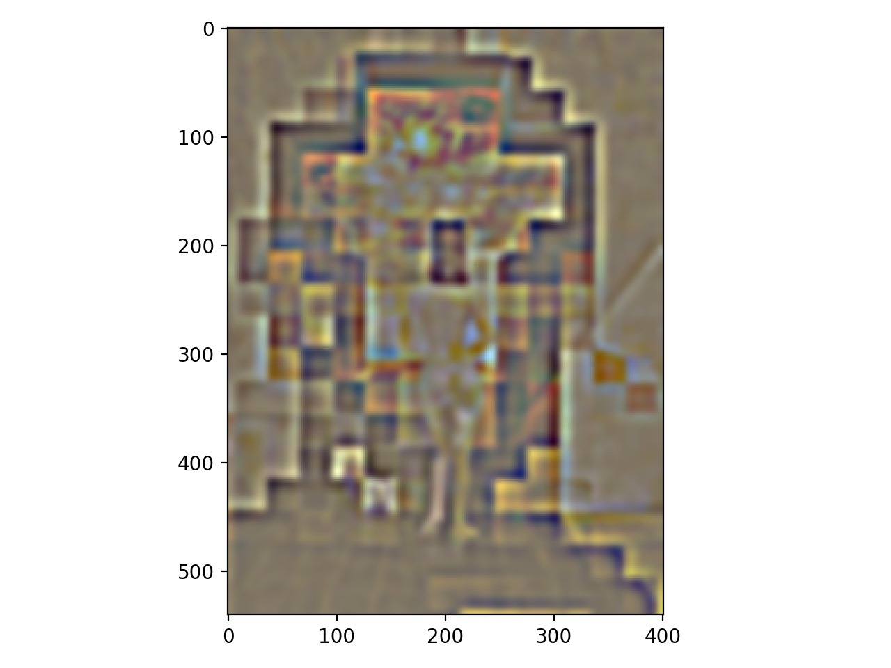
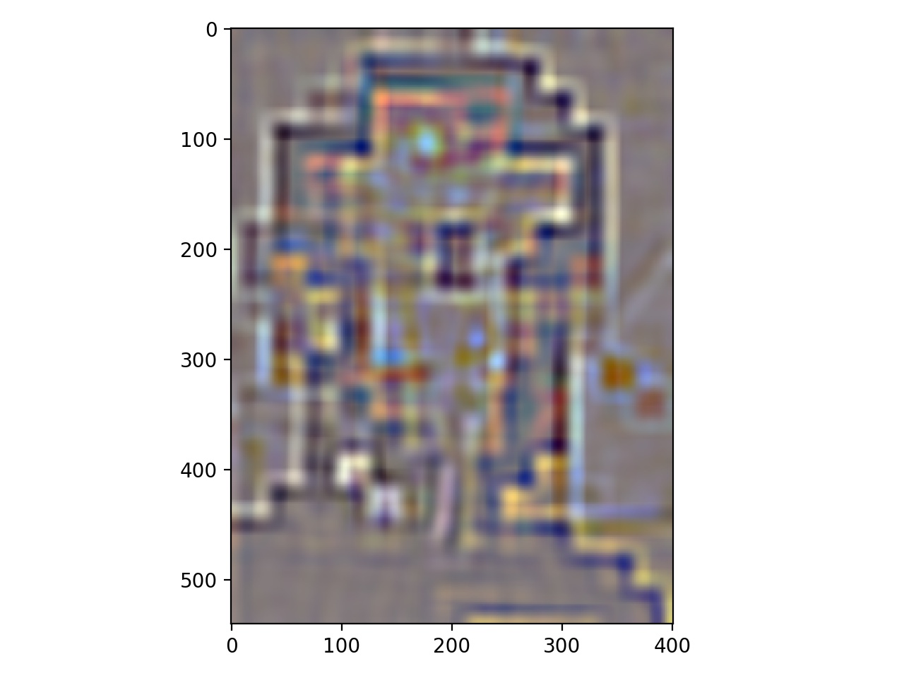
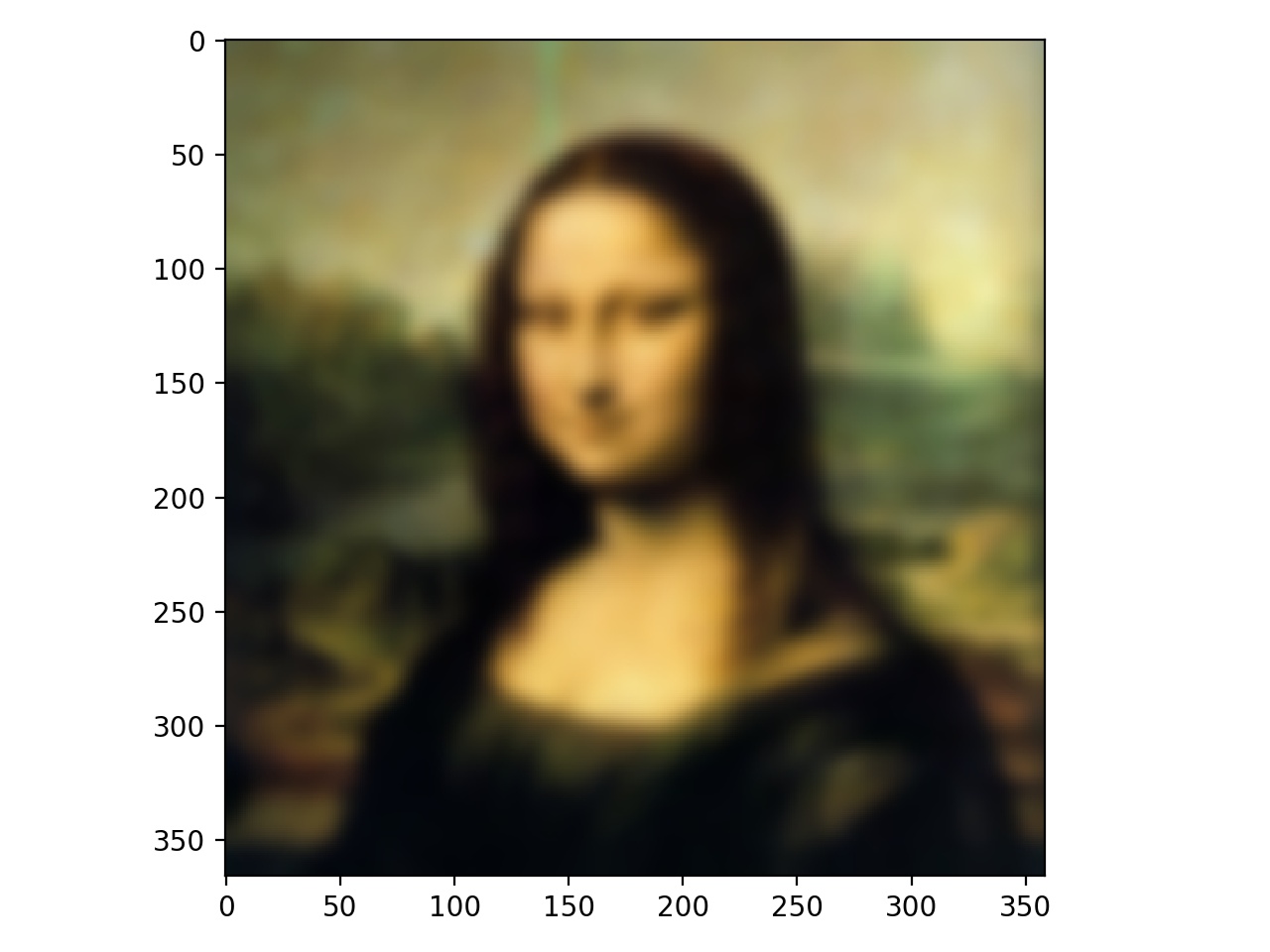
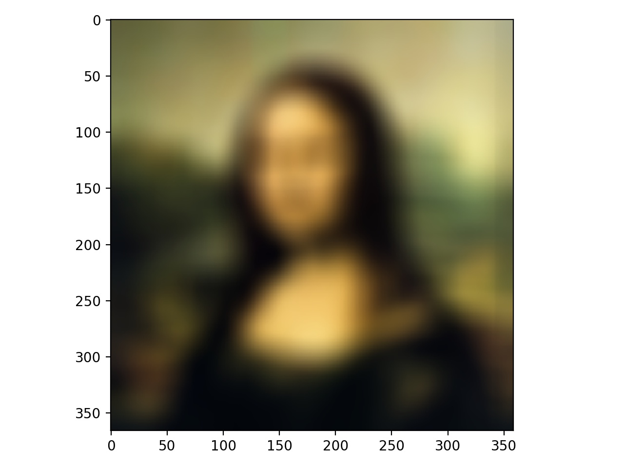
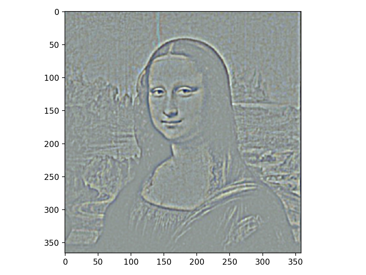
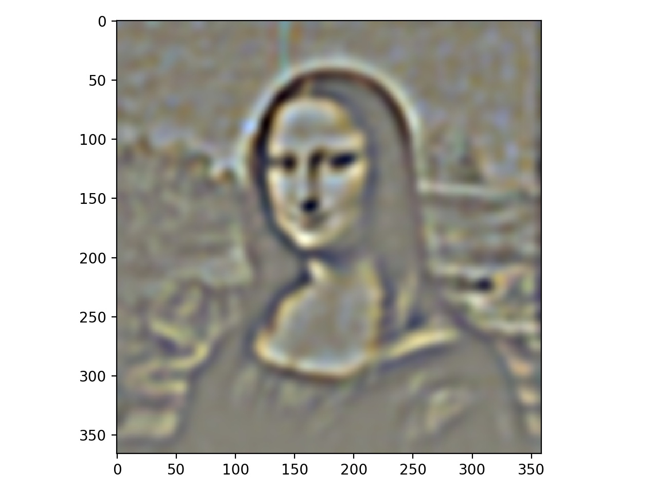
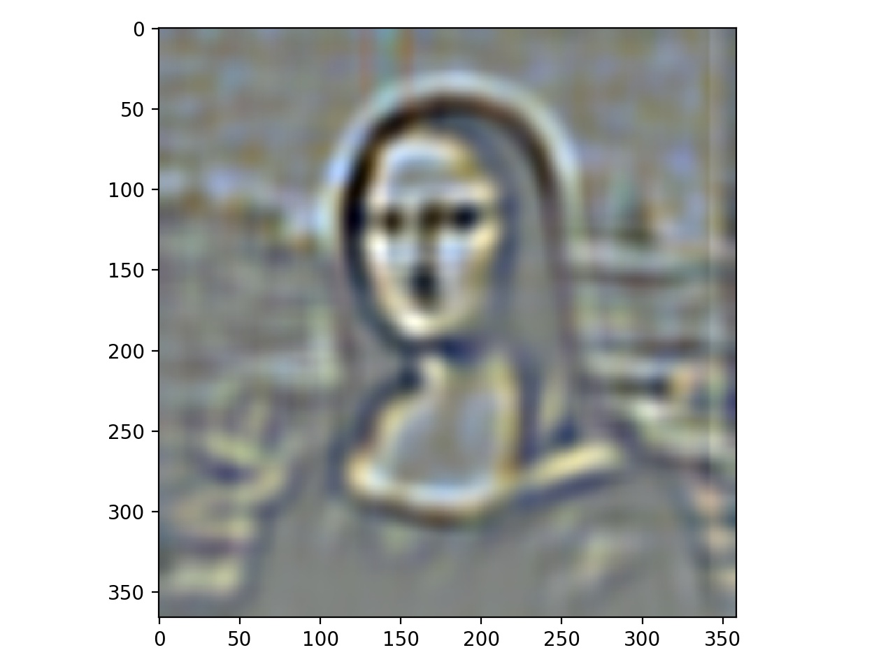
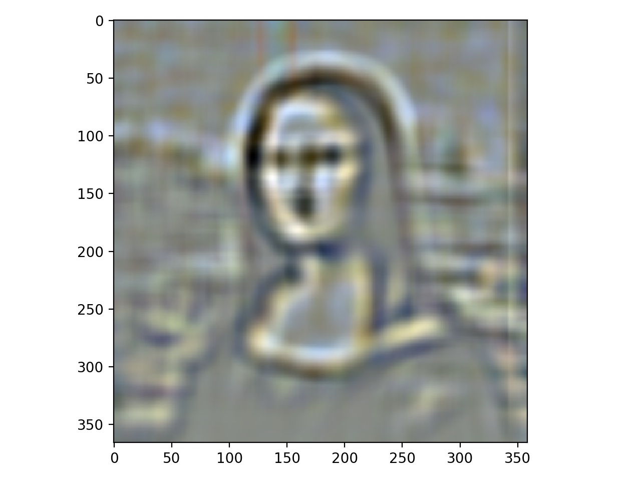
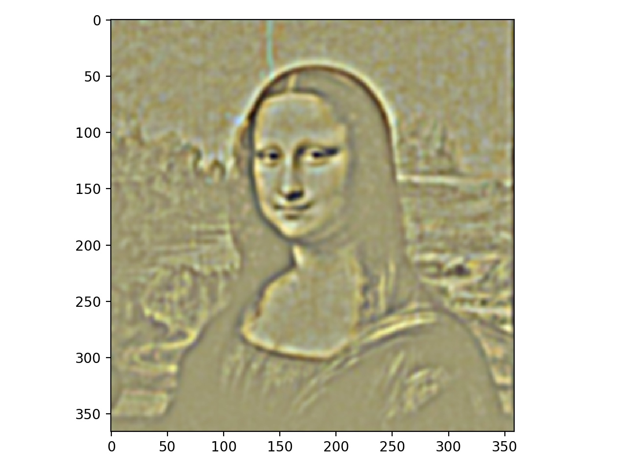
We can also make stacks of images that display different frequency content of an image. In a gaussian stack, we convolve with a gaussian at each level, so each successive image has a smaller active frequency range, in the low frequencies. In the laplacian stack, we take the difference of the images in the gaussian stack, and store them. Therefore, the images are band-pass filtered versions of the original. In a laplacian stack,we also store the most low-pass image to retain all the information in the original image. We first examine gaussian stacks of the Mona Lisa and Dali's painting of Lincoln and Gala to see different frequency level content. We display the laplacian stack in grayscale because it is easier to see the different bands.
Lincoln Gaussian Stacks
Lincoln Laplacian Stacks
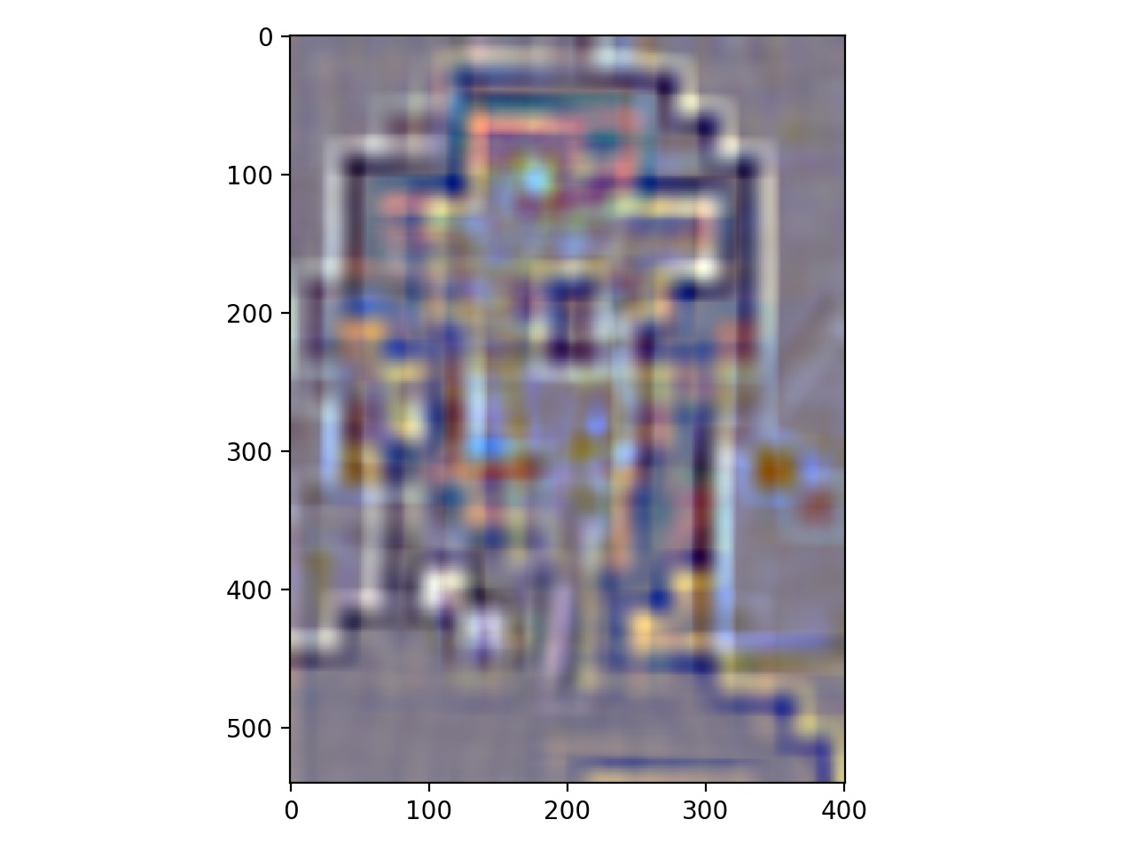
Mona Lisa Gaussian Stacks
Mona Lisa Laplacian Stacks
Vivek's face Gaussian Stacks from Vivdroid
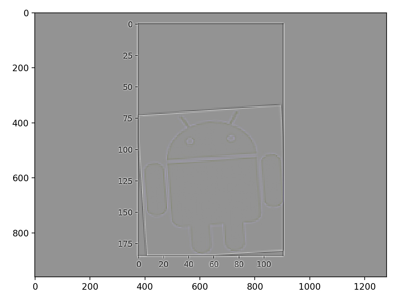
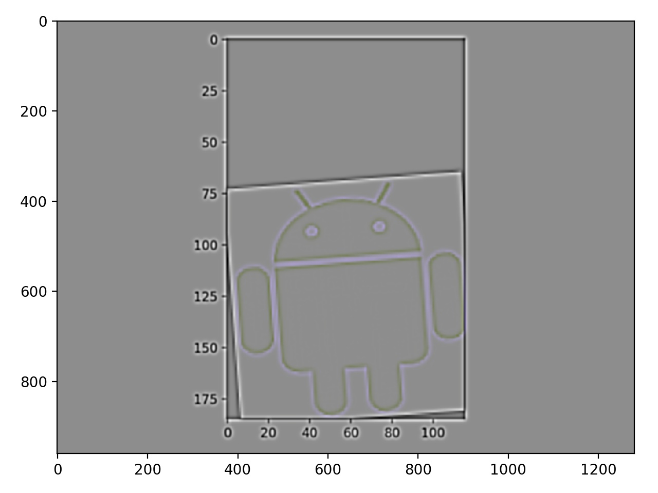
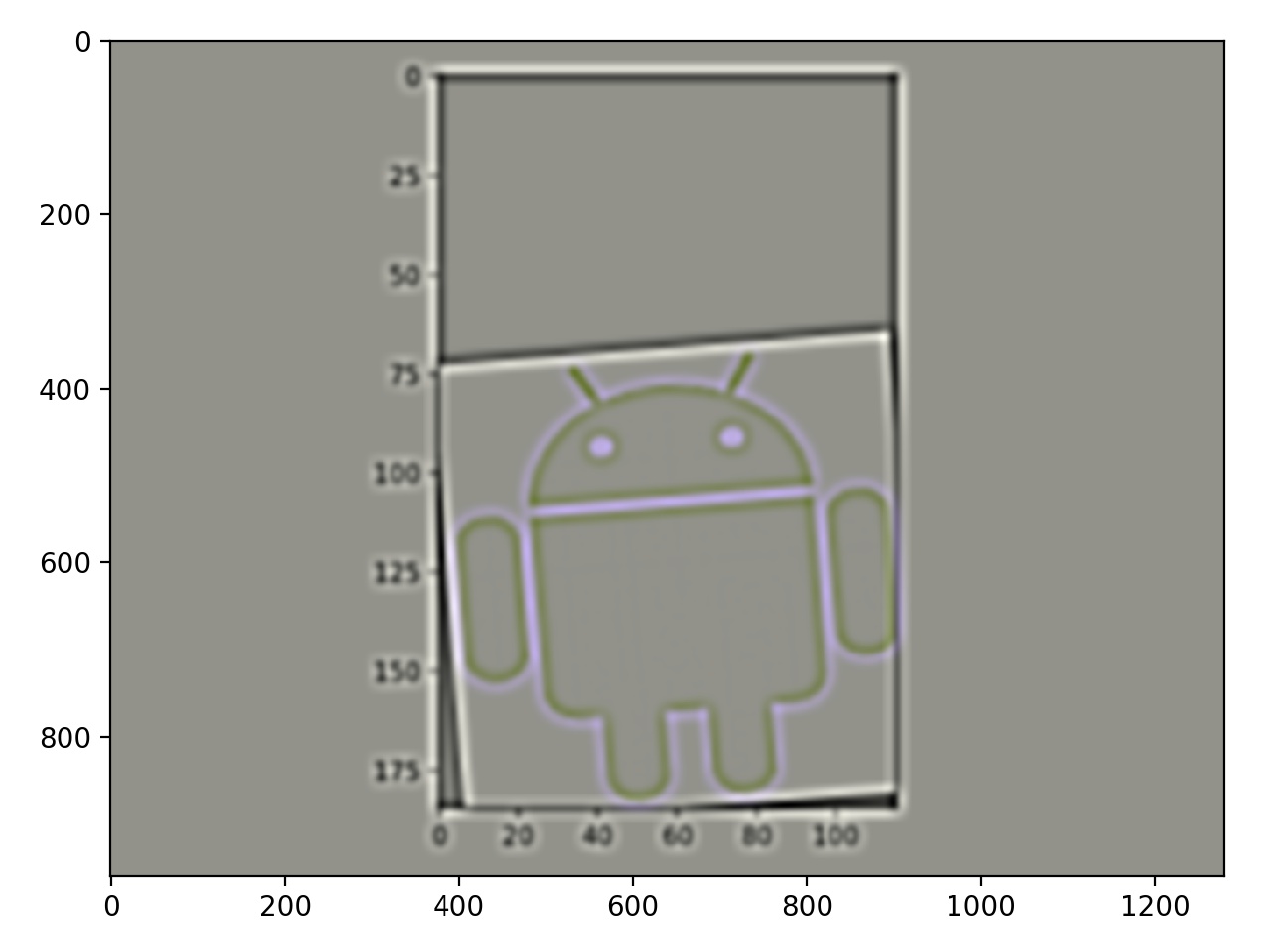
Android logo Laplacian Stacks from Vivdroid
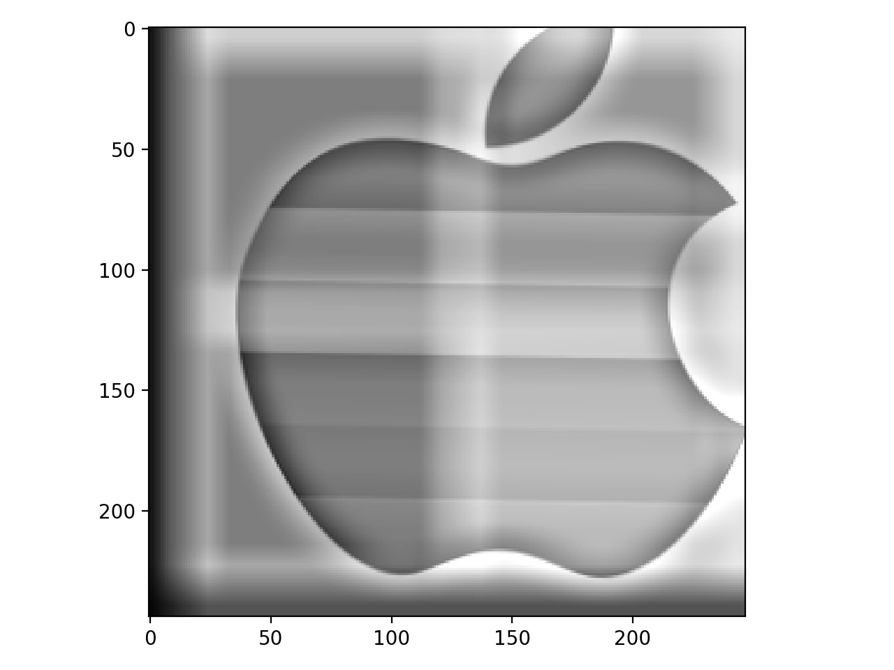
Part 1.4: Multiresolution Blending
We can use these stacks to also perform more seamless blending by blending together images at different frequency bands, and then compositing the result. Here are some examples!
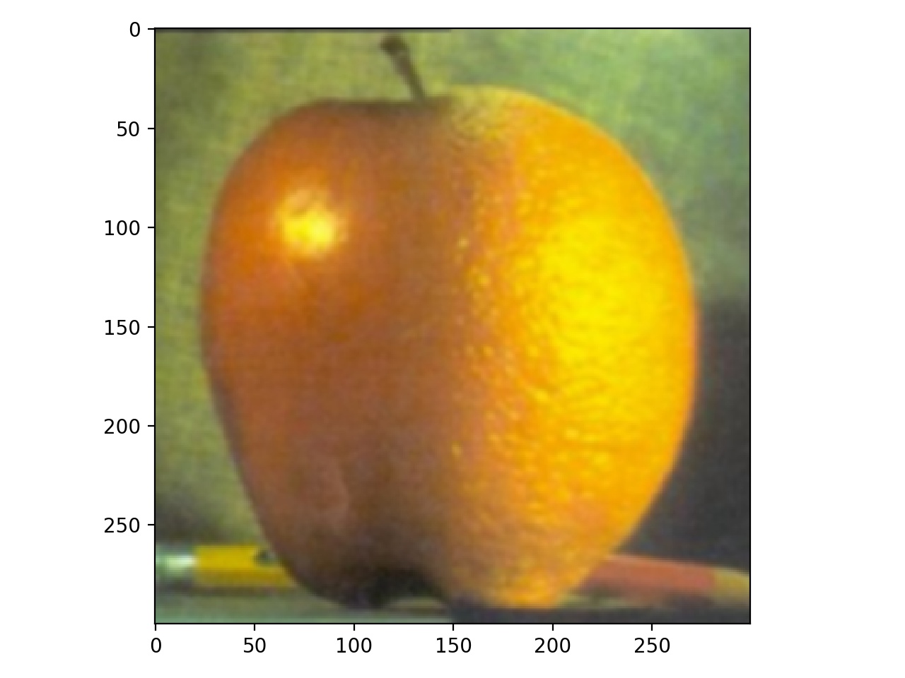 Orapple
|
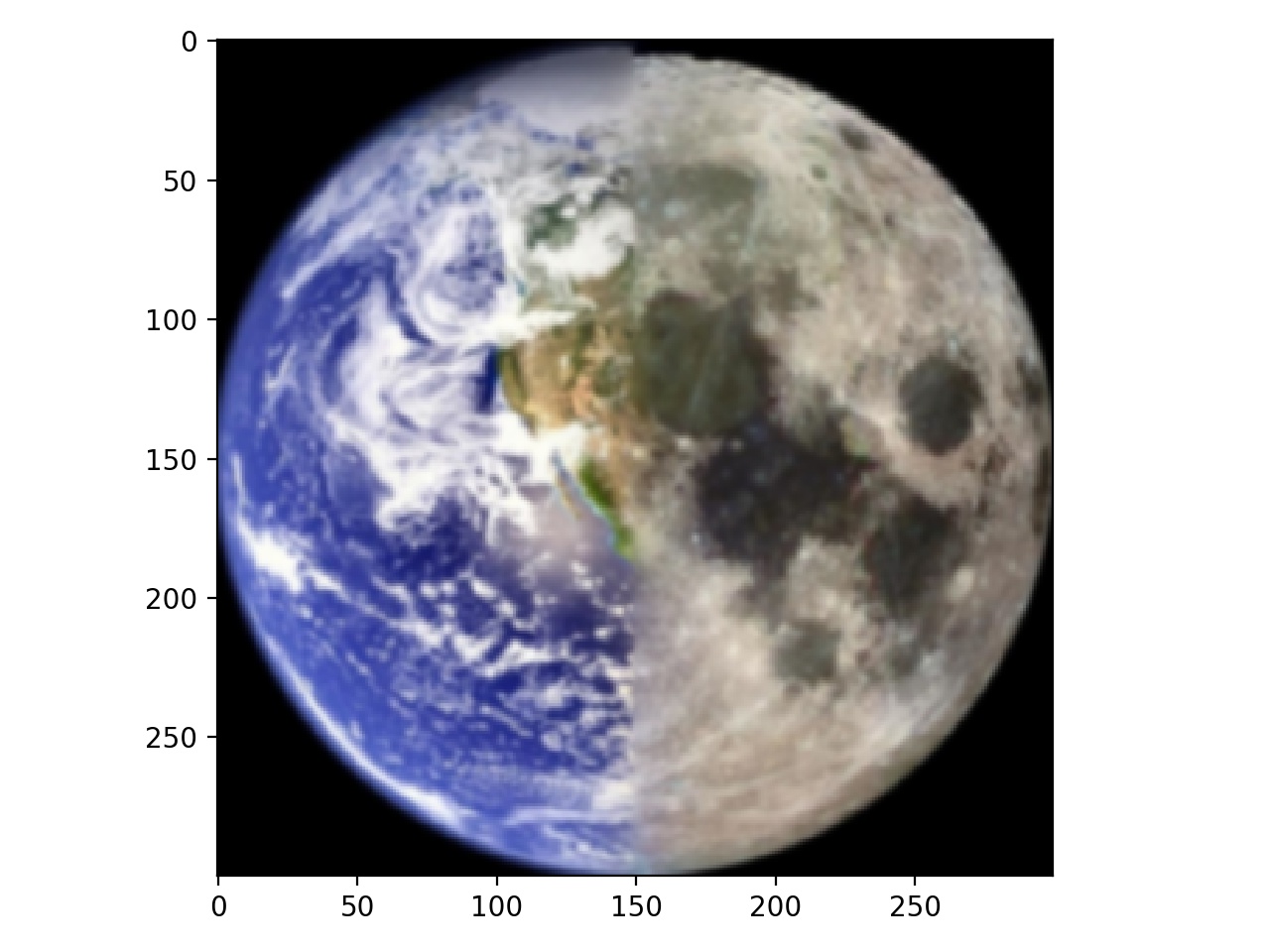 Dark side of the Earth...Moon? Ermoon?
|
 Mask used for orapple and ermoon(half black/half white)
|
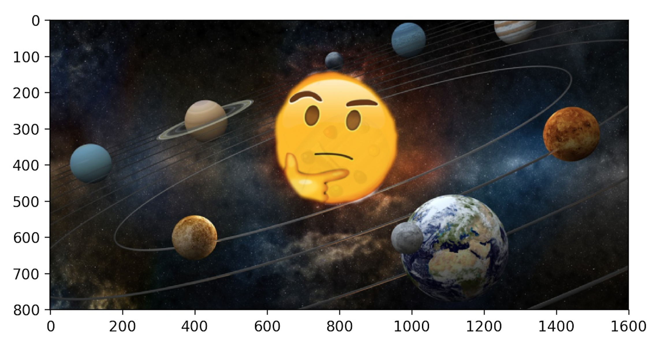 What are my planets up to today - sun
|
 Irregular Mask used
|
Part 2: Gradient Domain Fusion
Gradient Domain Fusion is a technique for blending images that allows image transplantation by transferring the gradient representations of a source image to a target. We can approximate taking part of an image and appending it into another by minimizing the different in gradients in the source and target images.
Part 2.1: Toy Problem
In this first section we perform an optimization on a single image to solve the toy problem. Performing this correctly means we get the same image back. As shown below, I fed the original toy_image in and got the same image out after solving the toy problem.
 Original Toy Image
|
 Toy Image Out
|
Part 2.2: Poisson Blending
Poisson Blended Images results
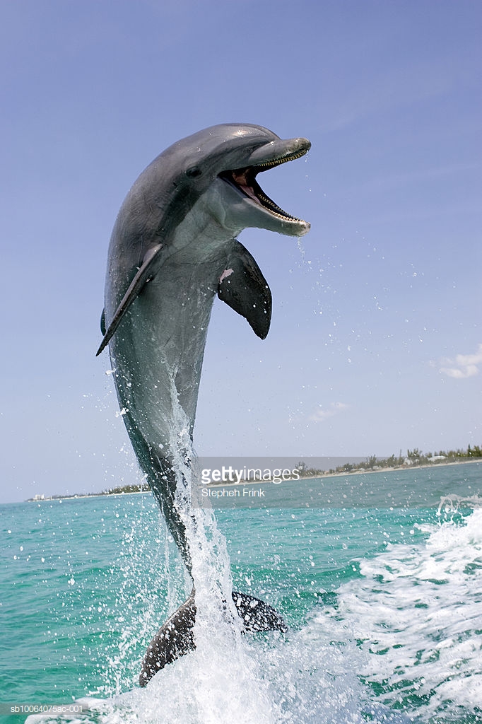 Original Target Image
|
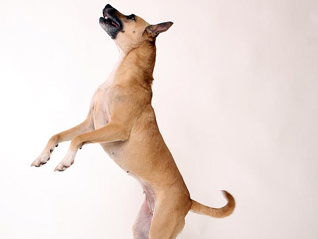 Orginal Source Image
|
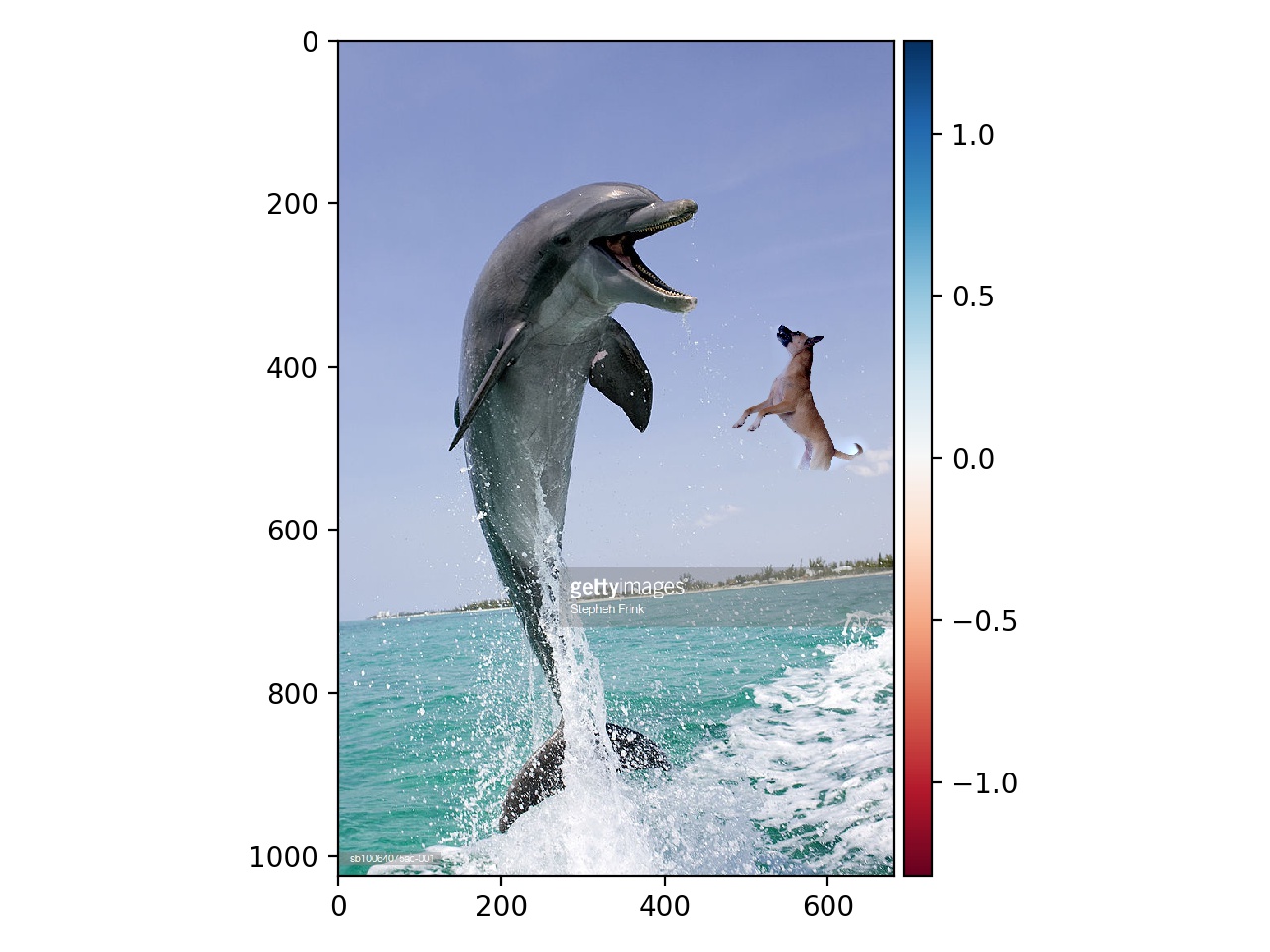 Poisson Blending Result - Doggo meets Dolphin
|
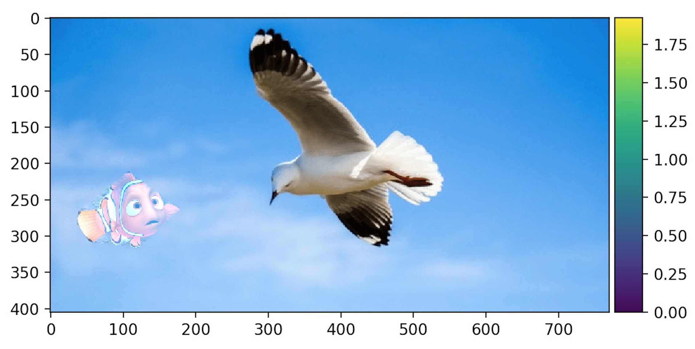 Poisson Blending Result - Nemo meets Bird
|
Failure Blending result
This is a failure case where we see discontinuities. This occurs because the empire state building is completely constant whereas the dinosaur is a very noisy and basically not apparent. We can't blend these easily together because there are alot of points. The pixelation of the dinosaur can also be because of the resizing of the image.
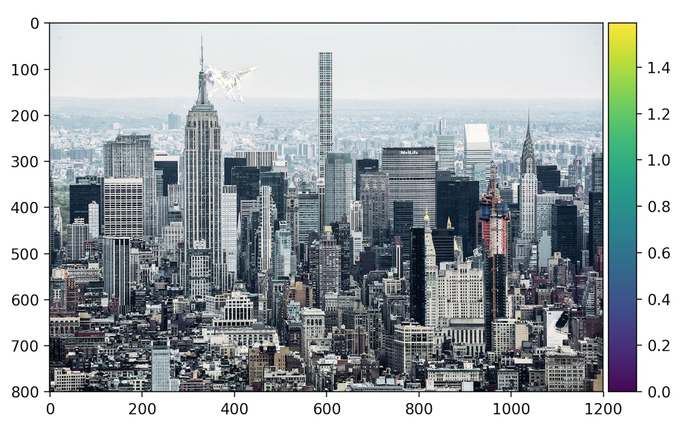 Failure to blend T-Rex with nyc skyline
|
Multiresolution Blending vs Poisson Blending
Here we compare the solar system and emoji blend from earlier to the blend using gradient domain fusion. The blend using gradient domain fusion works a lot better here because the borders between the sun and the emoji is a lot smoother - because we have to satisfy the boundary constraint. Moreover, this blend can be categorized more cleanly as a patch insertion.
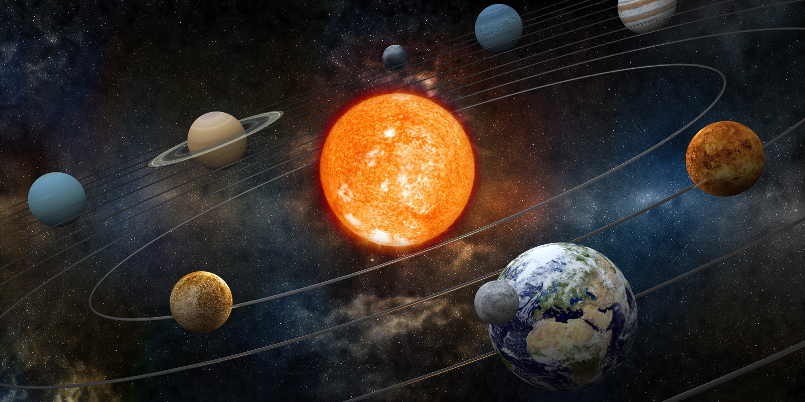 Original Target Image
|
 Orginal Source Image
|
|
Multireseloution Blending Result
|
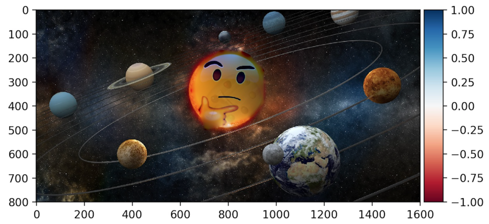 Poisson Blending Result
|