|

|
|
|
|
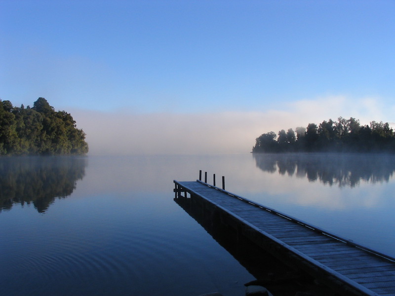
The purpose of this project is to explore different methods in blending images together.
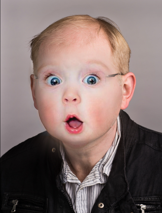
Using the unsharp mask technique: adding a scaled version of the image's high frequency content to the original image. I sharpened the following images with different alpha (scaling factor) values: 0.5, 1.0
|

|

|
|

|

|
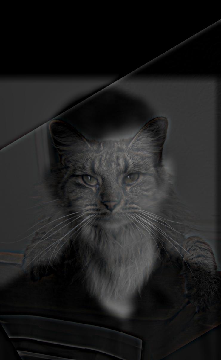
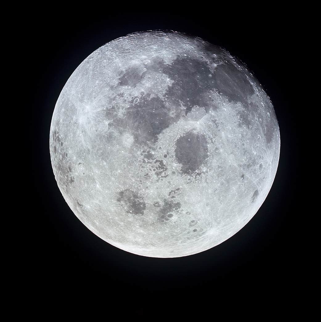
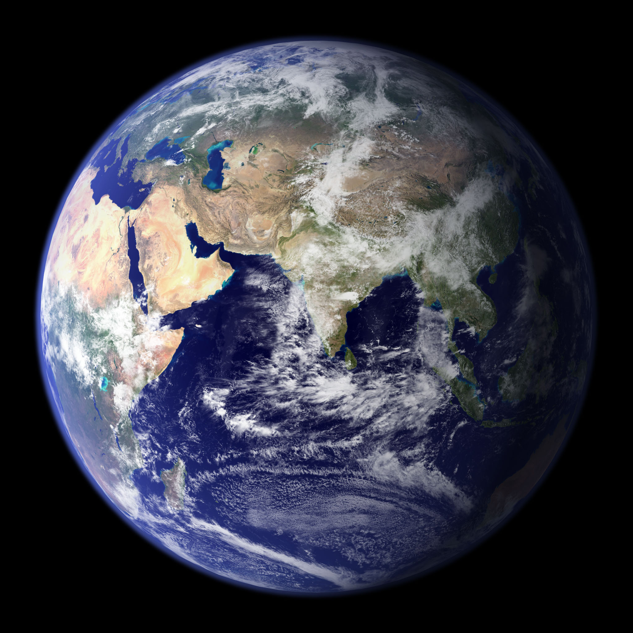
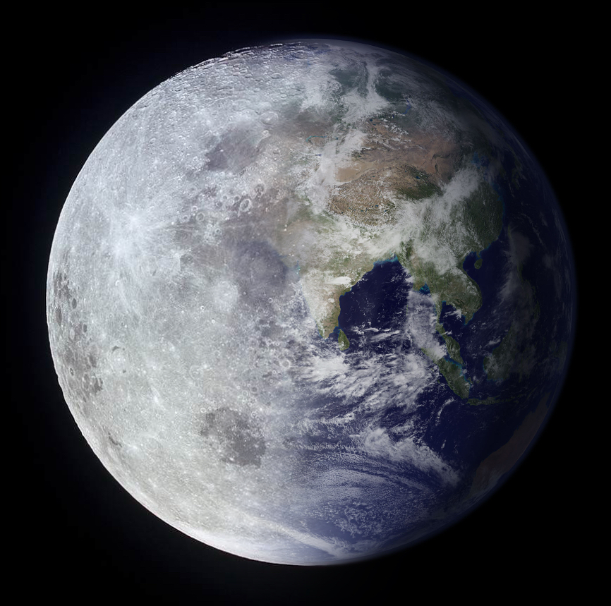
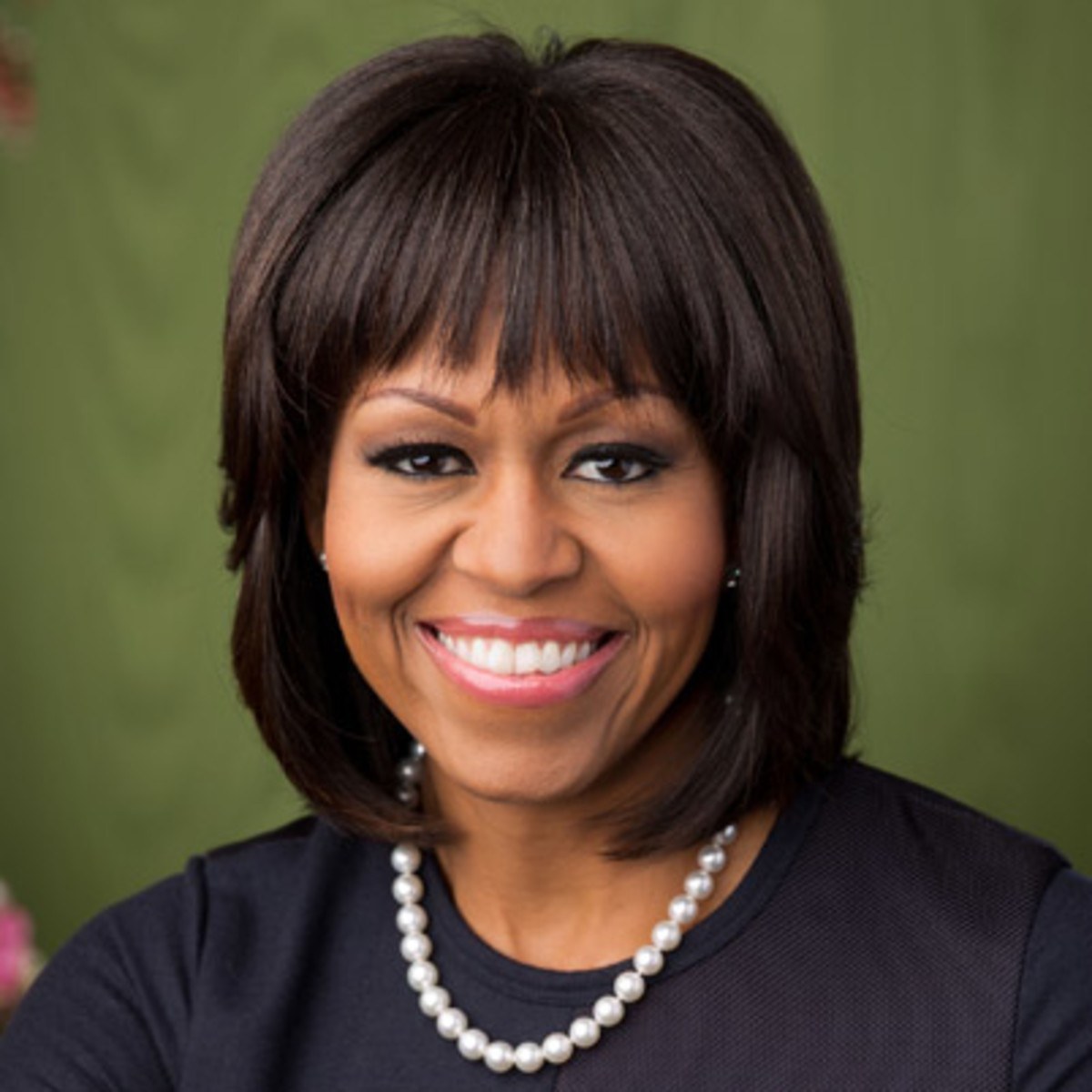
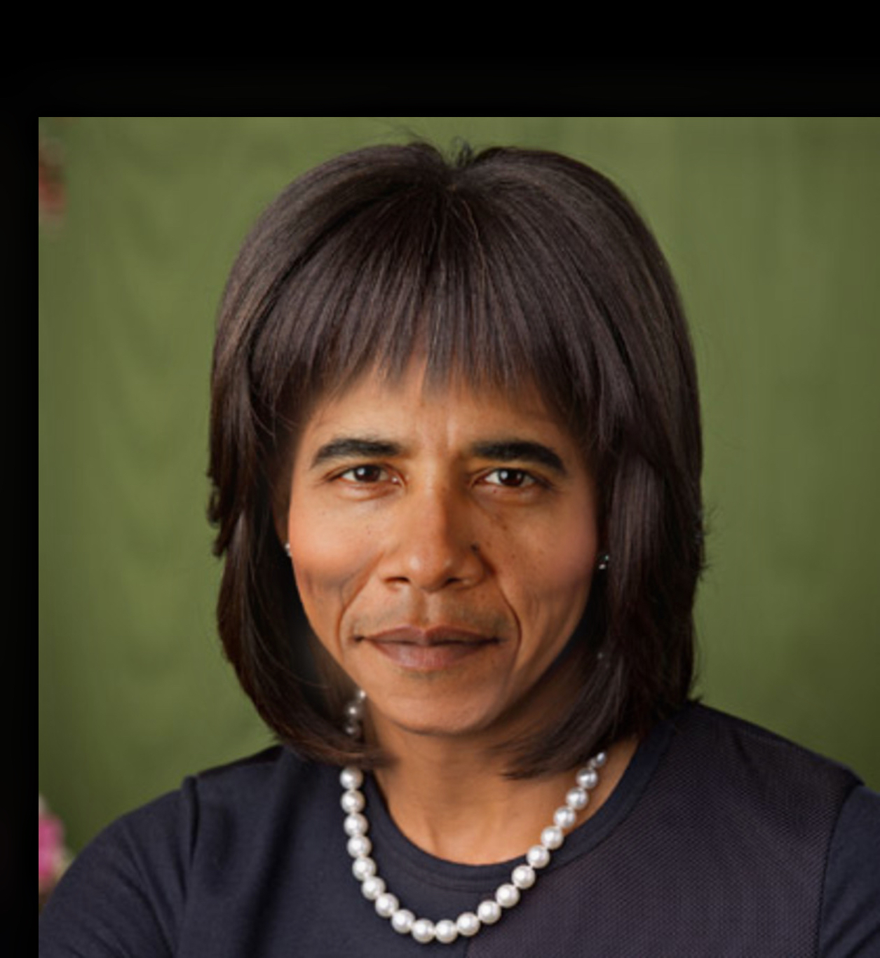
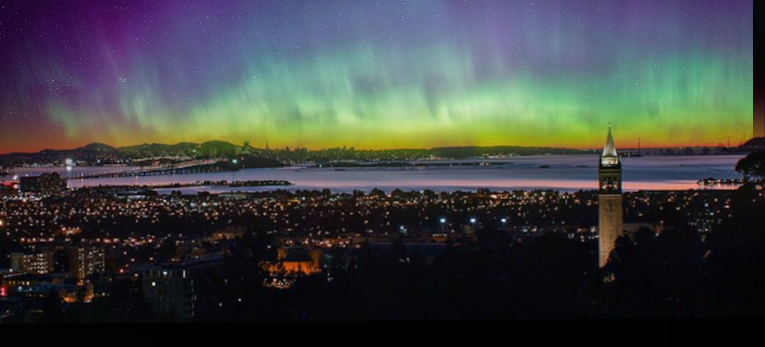
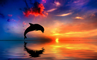
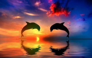
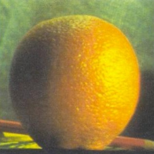
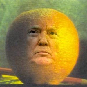
High frequency components of images tend to dominate our perception when viewing an image up close. At a distance the low frequency components of an image become more prevalent to our perception. We can blend the high and low frequencies of different images such that they can be percieved differently with the distance from which they are viewed. All of the following images were generated using kernel size: 31 and sigma: 15 for the gaussian filter.
|

|
|
|
|

|
|
|
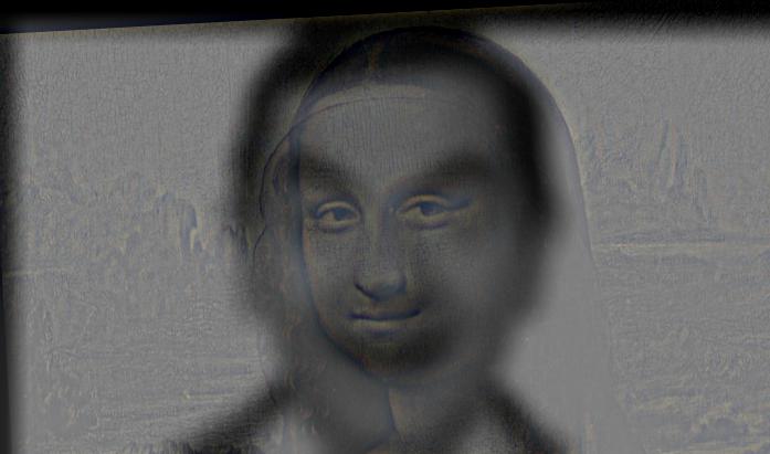
Unfortunately in the above images the high frequencies of Mona Lisa were not displayed very prominently, making her hard to see with Mr. Bean in the background.
Hybrid with Color: I found that depending on the image some images looked better with both frequency components colored whereas some looked better with just the high frequency components colored

|

|
|
|
|
|
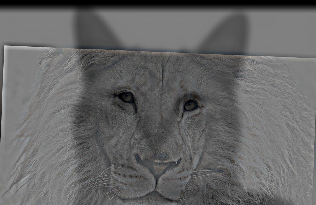
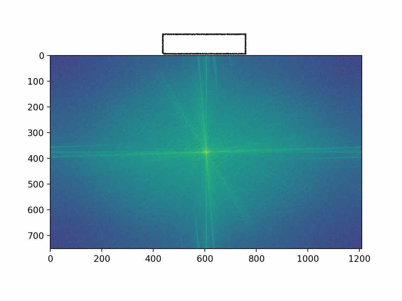
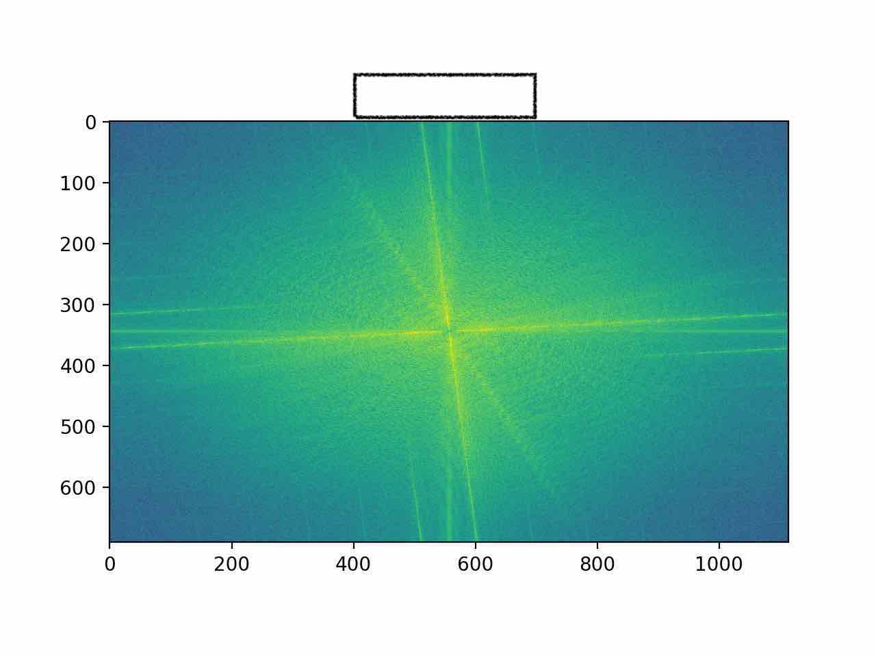
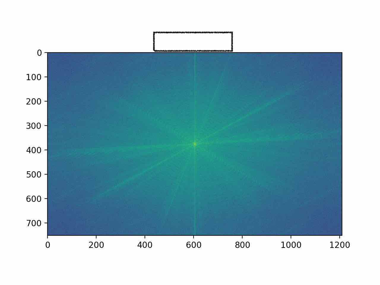
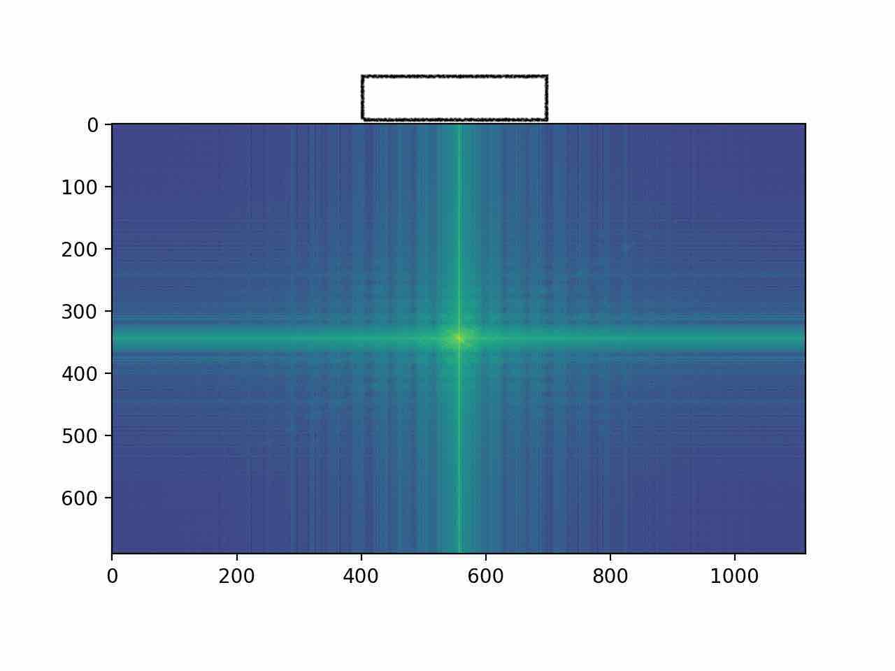
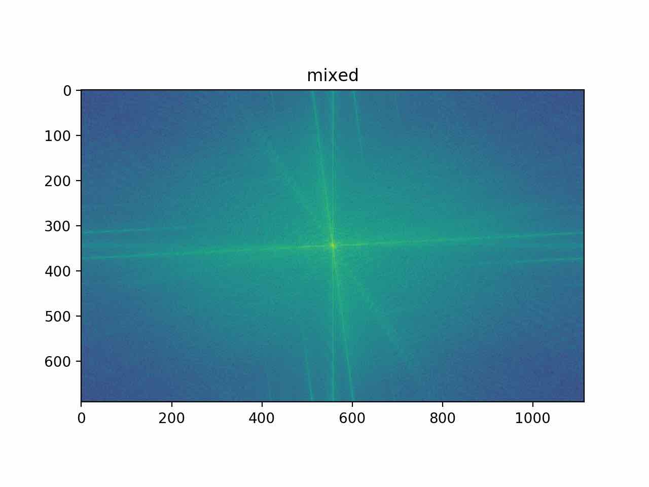
Let's now analyze some of the images by looking at the log magnitude of their 2d Fourier transforms. I performed the following on the hybrid image of Rick and Morty.
|
|
|
|
|
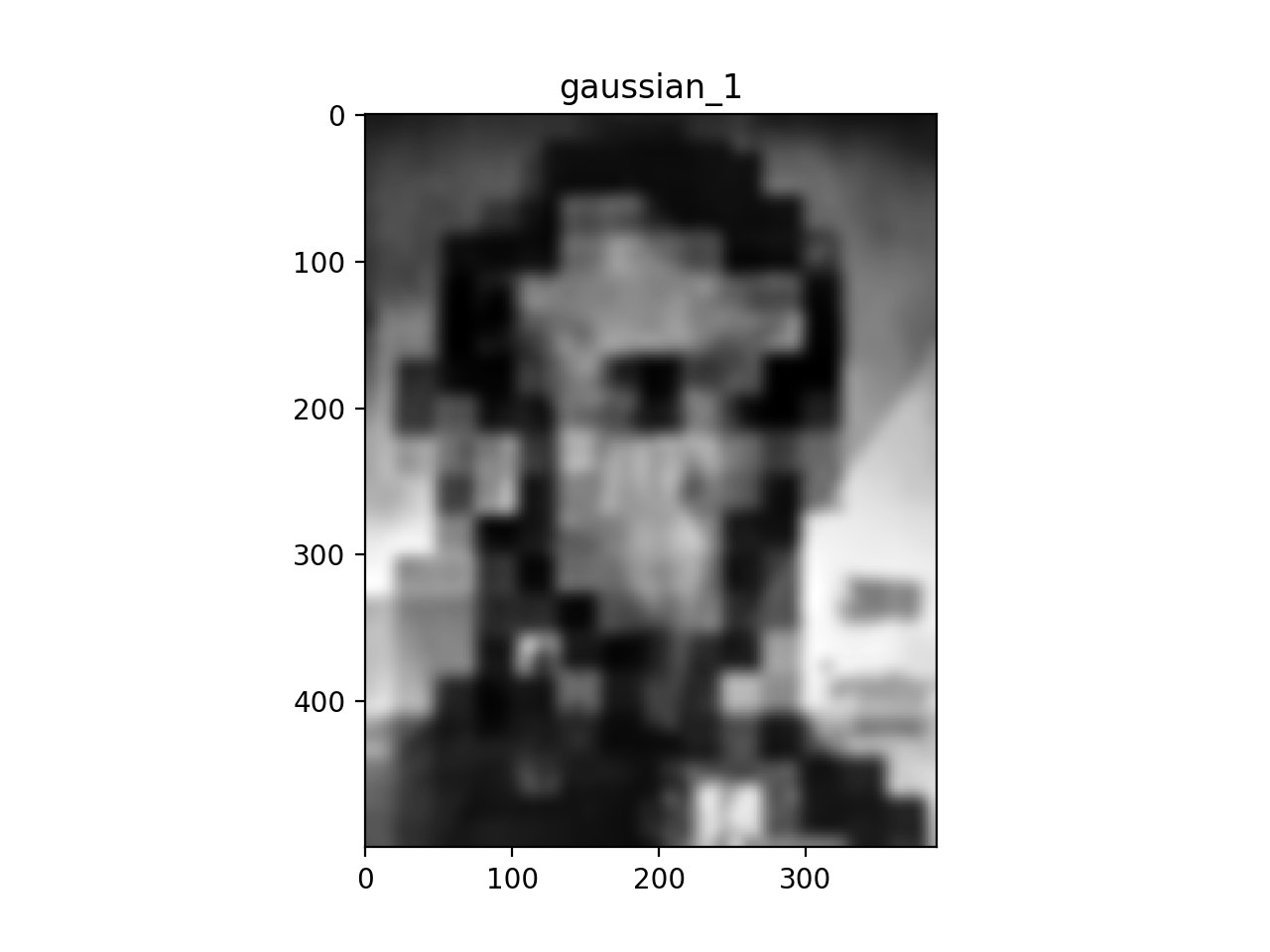
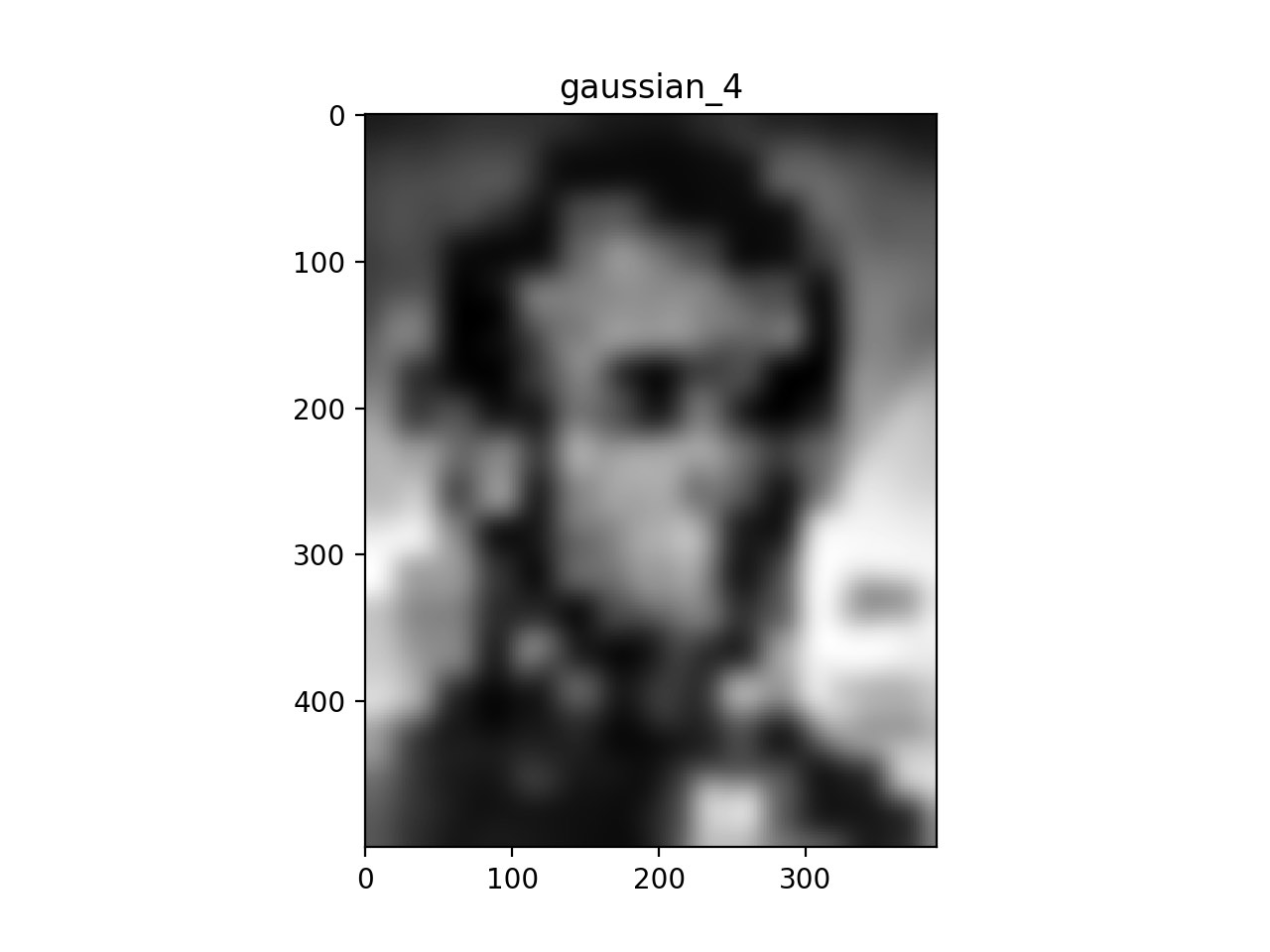
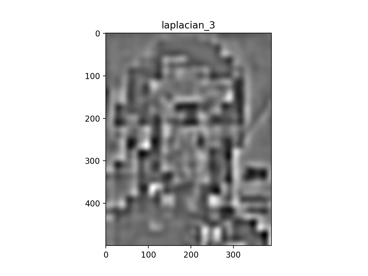
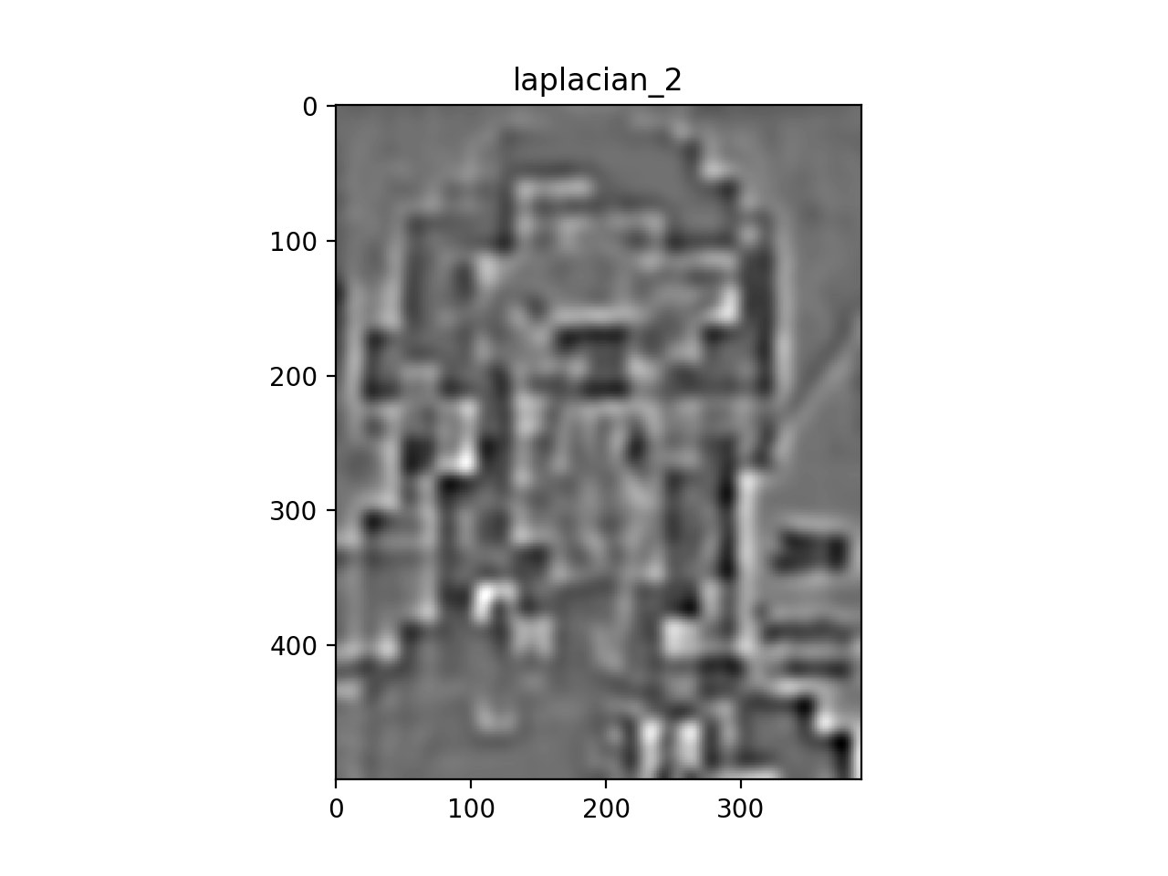
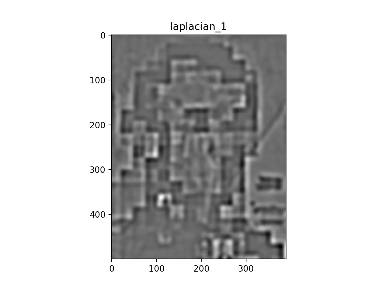
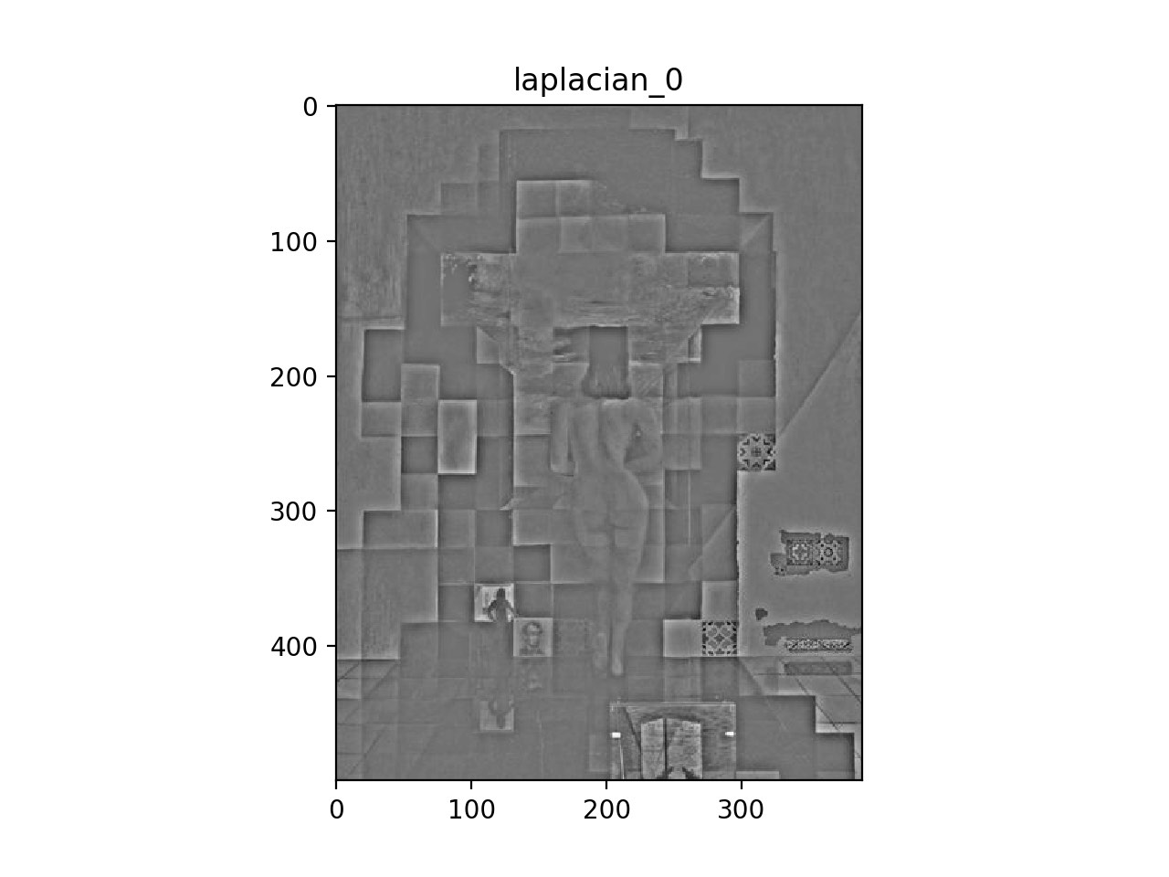
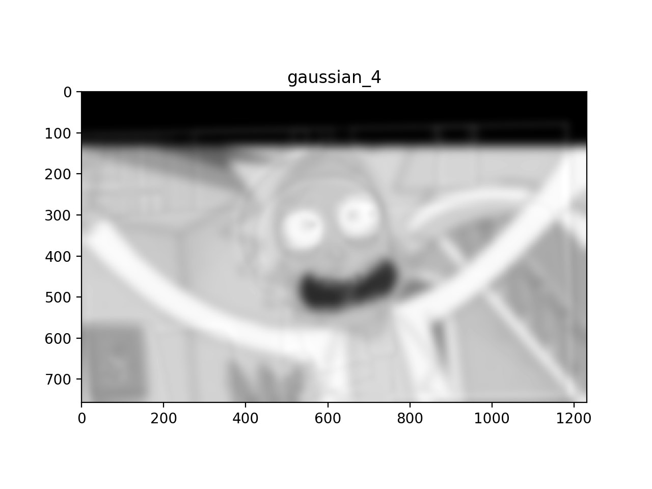
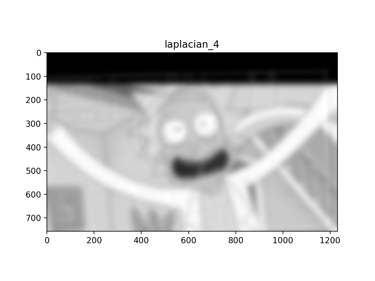
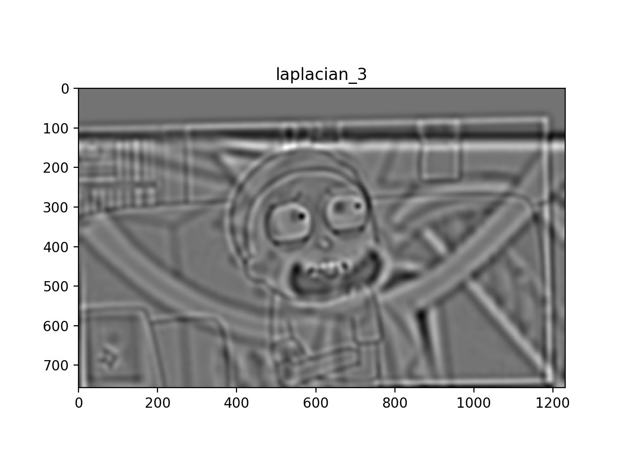
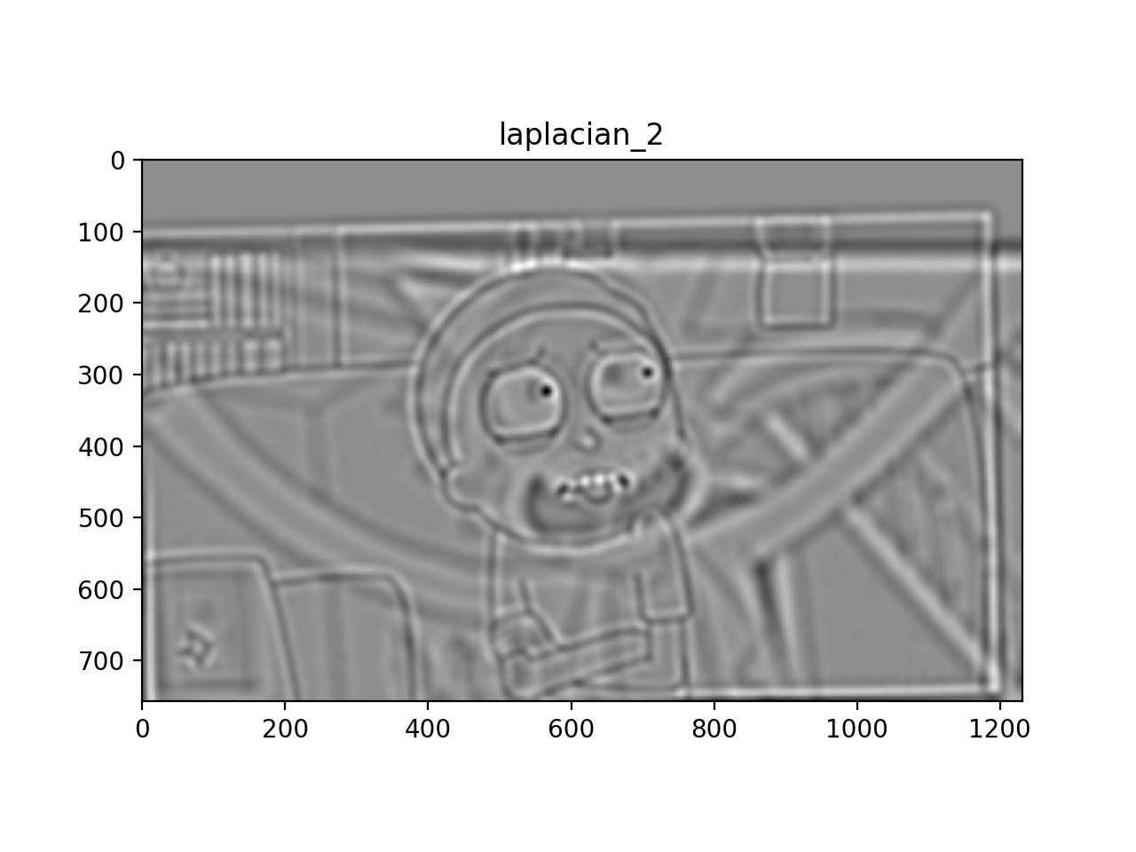
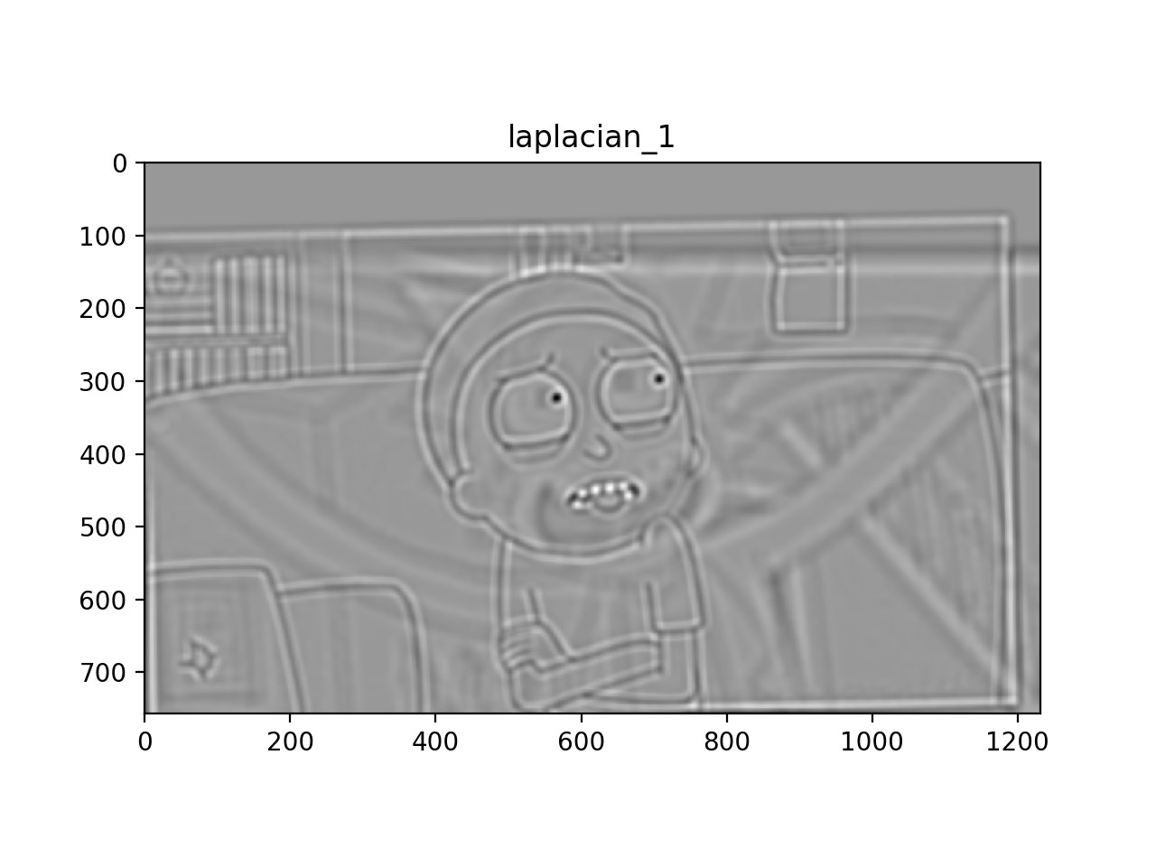
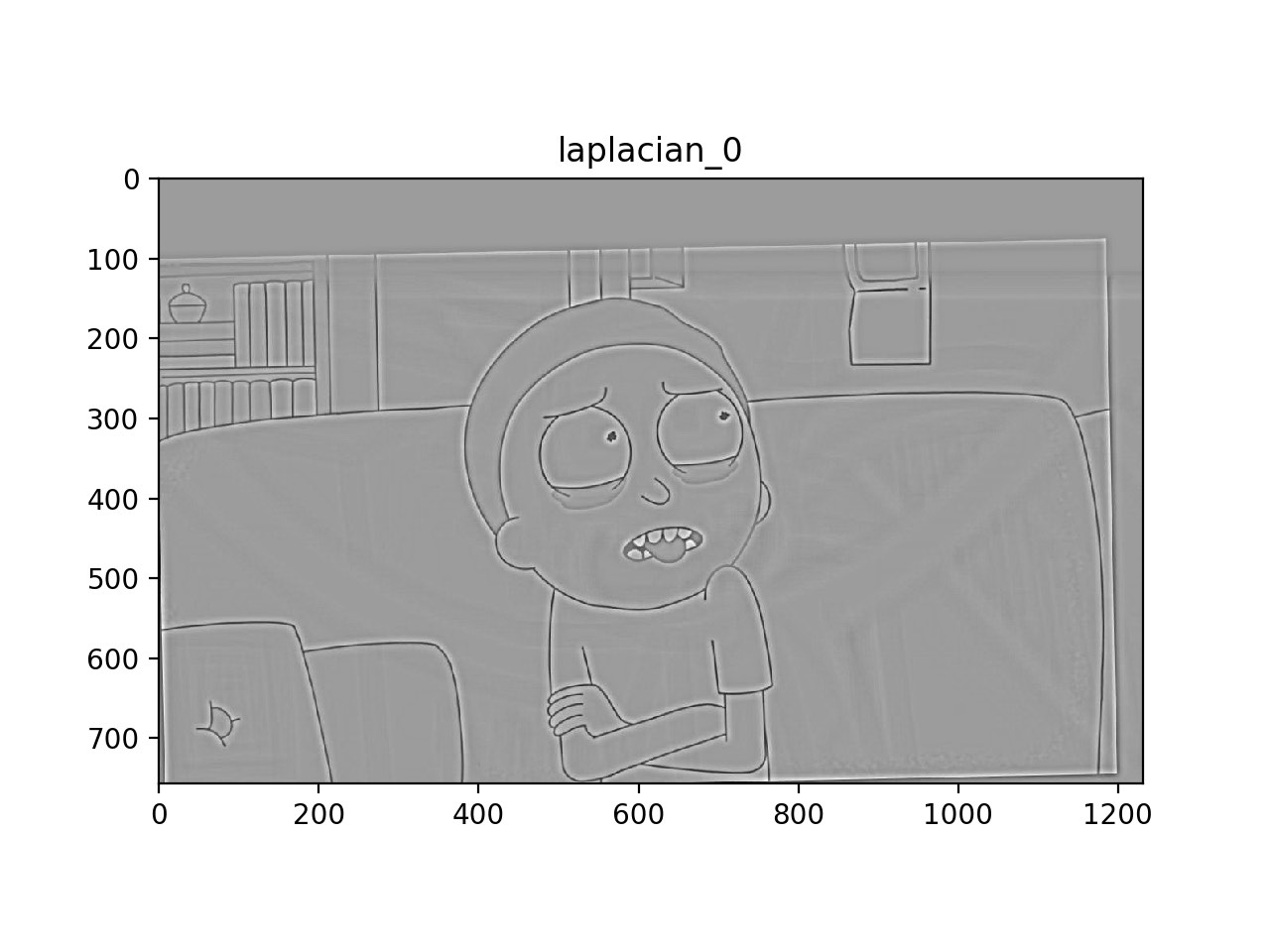
To help us further analyze the images we can compute the gaussian and laplacian stacks of the images. By blurring the image the gaussian stack lets us easily visualize the low frequency content of images. Equivalently the laplacian stack acts as a high pass filter helping display the high frequency content of the images. The stacks were generated in grayscale with 5 layers a kernel size of 21 and sigma of 5 for the filters.
Let's start by analyzing Dali's Gala Contemplating the Mediterranean Sea Which at Twenty Meters Becomes the Portrait of Abraham Lincoln. Notice how it becomes easier to see Lincoln in the gaussian stack and easier to see Gala in the laplacian stack
|

|

|
|

|

|
|
|
|
|
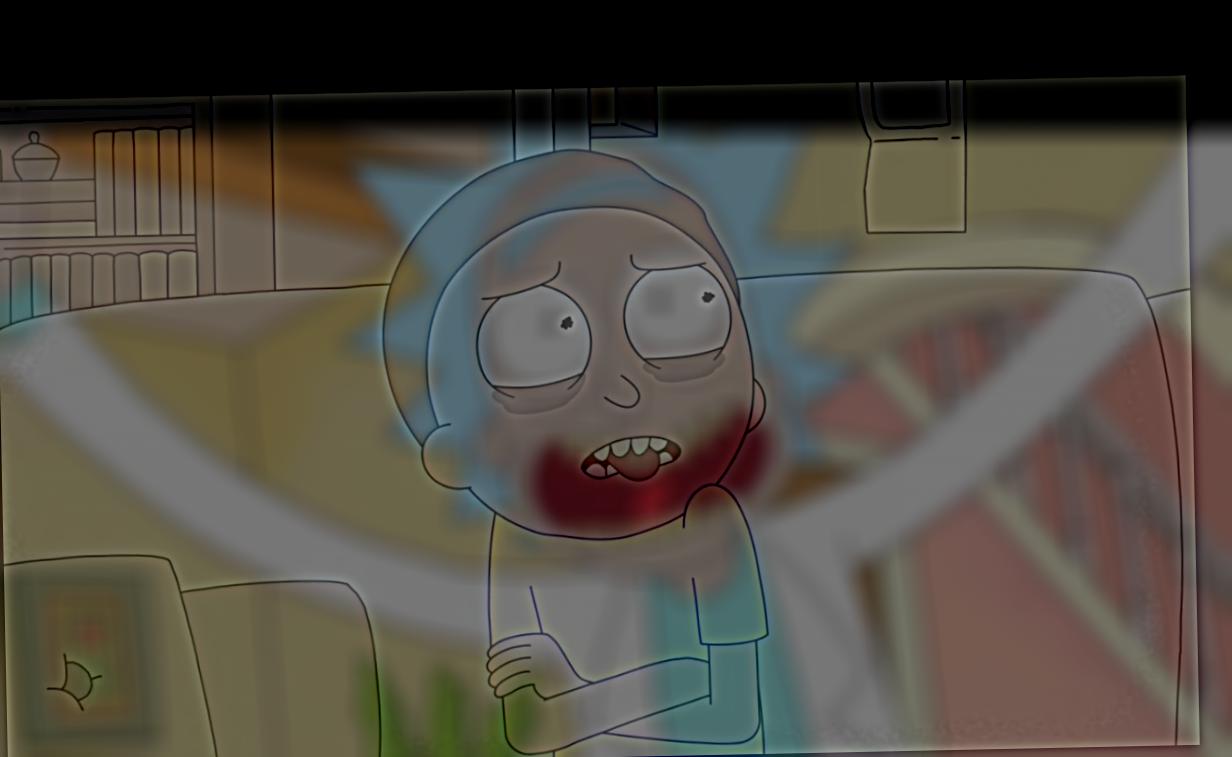
Let's now analyze the rick and morty hybrid image using laplacian and gaussian stacks. Notice how it becomes easier to see rick in the gaussian stack and easier to see morty in the laplacian stack.

|

|

|
|

|
|
|
|
|
|
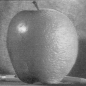
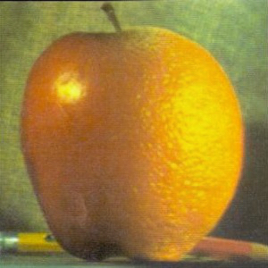
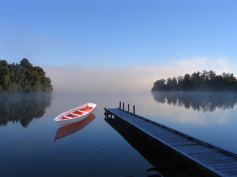
We now use the laplacian and gaussian stacks that we implemented to create a naive blending algorithm. To blend two images together we first create a mask. We then make a gaussian stack of the mask and make laplacian stacks of the source images. We use the gaussian stack of the mask to blend together the laplacian stacks of the two source images. The sum of the blended laplacian stacks is the final result. The images were generated using 3 layers, a kernel size of 75 and sigma of 35 for both the gaussian and laplacian stacks.
|
|
Now that the multiresolution blending was working I experimented with more complex masks to get better results (Bells and whistles: I utilized color for the laplacian blending).
|
|
|
|
|
|
|
|
|
|

|
|
|

|
|
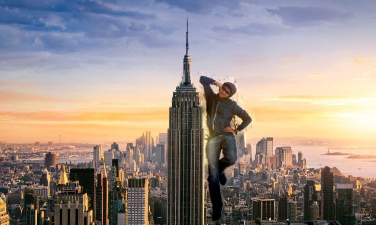
Up until now we were using frequency based approaches to blend different images together. However now we move on to take another approach. Being humans we are sensitive to abrupt changes in images, thus when performing blending operations we want to prevent these abrupt changes as much as we can. To do this we turn to gradients which are multidimensional derivatives that describe changes in the pixels of the images. Our goal is we want to preserve the gradients of the source image that we are blending, within a specific region of the target image however to prevent an abrupt change we want the gradients of edges in the target image to flow seamlessly into the blended source image area.
We frame this as an optimization problem that can be solved by least squares to find the value of each pixel in the blended area.
We use the above described gradient approach to reconstruct a toy image from just one pixel. By treating the whole image as the source area that we want to recreate we can create a series of equations using x and y gradients. We then use one pixel of the image as an initial point to solve for the pixel values of the image letting us recreate the toy problem with an error of: 5.412851648810523e-13!
|

|
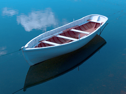
We now employ the above described technique to blend images together. Though this yields decent results doing least squares on such large images is very computationally intensive:
|
|
|
|
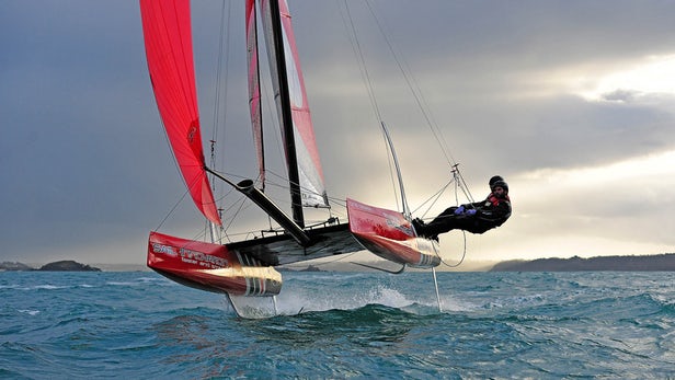
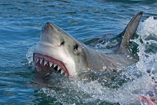
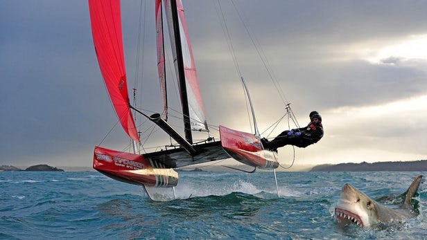
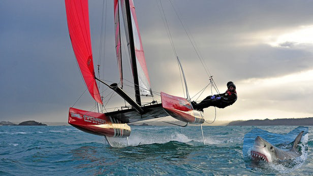
Here we can see that poisson blending uses gradients to integrate the shark much better into the target image than directly copying over the pixels from the source to the target image. This works as described above. After generating a mask we develop a matrix using the gradients of the pixels from the source image within the mask and gradients of the target image at the edges of the mask. We then solve for the pixel values within the blending region with a least squares operation. The matrix to solve this was quite large even for small blends, however knowing it was a fairly sparse matrix I was able to use a optimized sparse least squares solver to decrease computation time.
Failure Case: Some results were not as good as the image above. In the following image we see that since gradient blending does not preserve color it the blended image has an odd color tone. In addition to that since the source image had strong gradients surrounding the main object these gradients carry through to the target image making the blending seem less seamless as the blended image is surrounded by a halo of the old background.
|
|
|
|
|
|
|

|

|

|
|
|
|
|
|
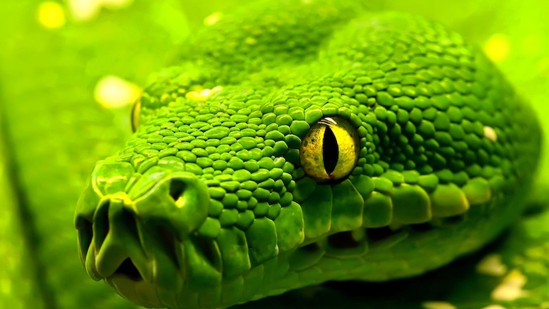
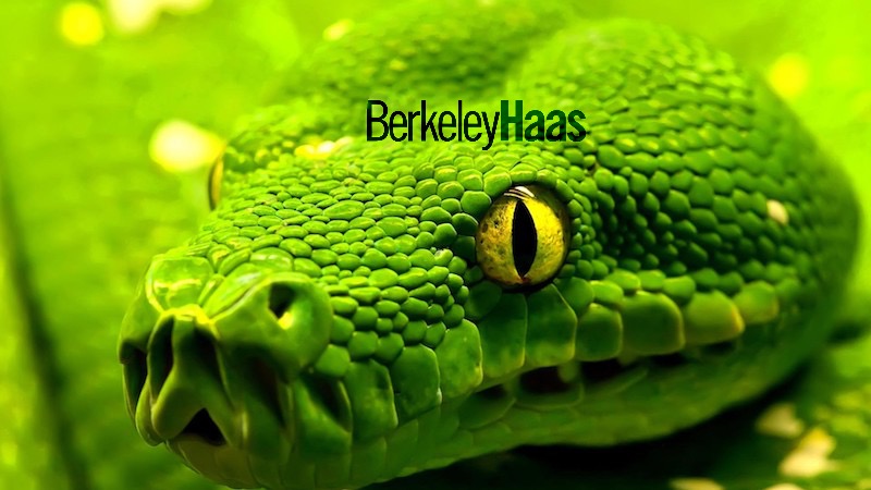
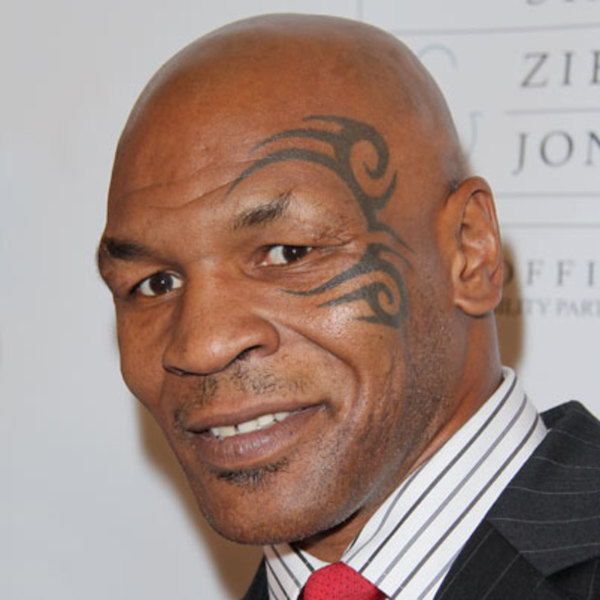
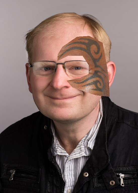
With mixed gradients we can weight the gradients coming from the source and target image. Here we take the stronger gradient of the 2. This allows us to take things like plain text and blend them into an image.
|

|
|

|
|
|

|
|
|
|

|
|
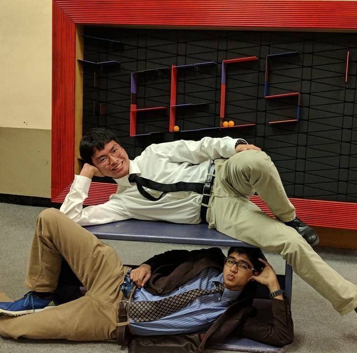
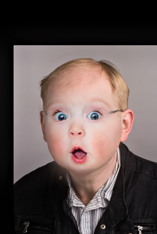
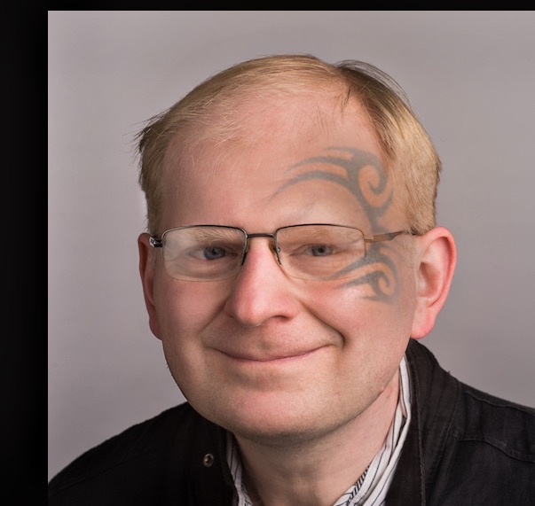
Here we can see that Laplacian blending does quite a good job but leaves the image looking strangely smeared. However as we saw from earlier this technique works well for blending faces and would have worked better if not for the difference in skin tones and with a slightly better crop (This method is also much quicker than the remaining approaches due to lower computational complexity). With poisson blending the results take care of the skin tone difference however since Professor Efros has glasses the glasses get covered making the image look unnatural. The best results are from mixed gradients. Here we get the advantage of poisson blending in that the skin tone of efros is preserved but since we take the highest gradient of the two images the glasses are preserved making the tatoo look much more natural.
Website template inspired by: https://inst.eecs.berkeley.edu/~cs194-26/fa17/upload/files/proj1/cs194-26-aab/website/