Alex Jiang
CS 194-26: Project 3
Fun with Frequencies and Gradients!
Overview
This project is where the heart of the course really comes into play, as we begin work with frequencies and gradients to perform substantial image manipulation. Through sharpening, reconstructing, hybridizing, merging, and blending, we discover many ways to enhance and change the nature of digital images in this project. It gets a little math-heavy, with plenty of reliance on numpy, but overall this was definitely one of the most fun projects I’ve done in a while :)
1.1 Warmup
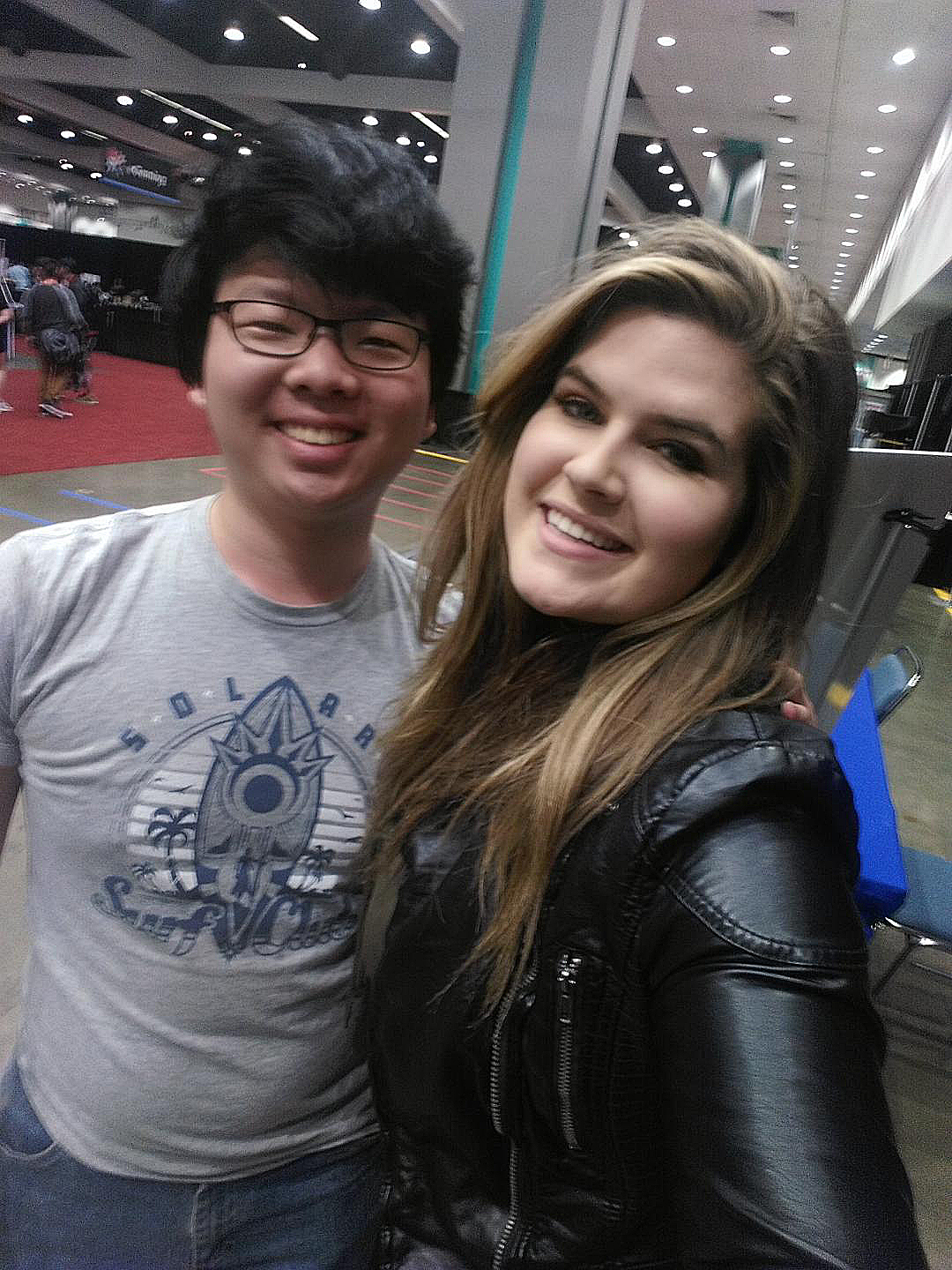
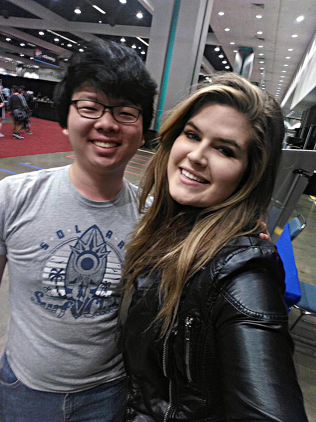
Original, Blurry | Sharpened | Gaussian Blur |
This picture was a slightly blurry selfie taken of me with voice actress Erica Lindbeck. A kernel was obtained via cv2.getGaussianKernel, and the image was subsequently blurred via cv2.sepFilter2D. Finally, cv2.addWeighted overlayed the blur over the original to create, the central sharpened version.
The picture does turn out to be notably grainy, which is to be expected as the individual particles in the image end up getting sharpened as well. The softer edges of hair did not improve as much of the rest of the image, as the edges weren’t rigid enough to be truly emphasized. Extreme blur, such as those of the people in the background, was preserved since the unsharp masking technique can’t get rid of such concrete issues. However, as a whole, the image appears noticeably sharper overall and shadows, in particular, seem much more clear. Throughout the course of this process, we are essentially identifying what counts as a “detail” through the use of the blur, scaling those accordingly and coming out with a more fine-tuned result.
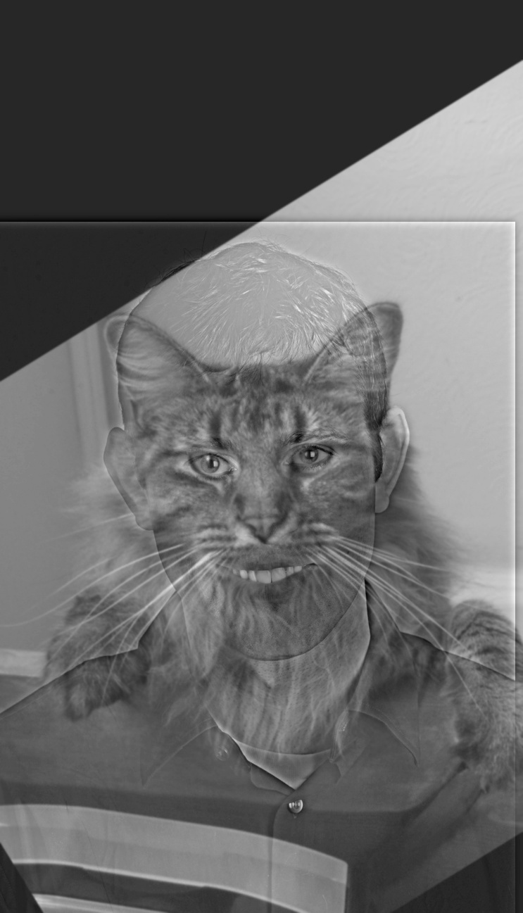
1.2 Hybrid Images
Derek (Σ=6) | Nutmeg (Σ=1) | Dermeg |
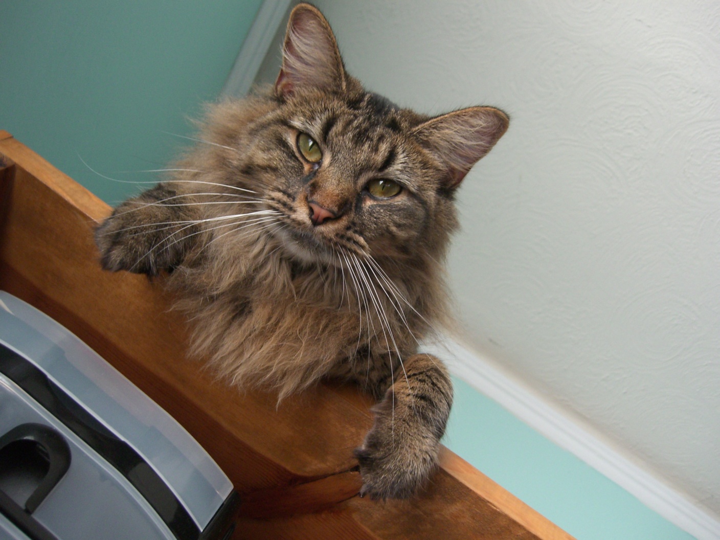
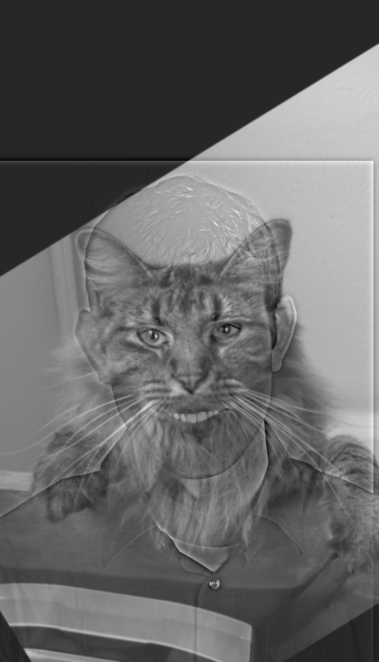
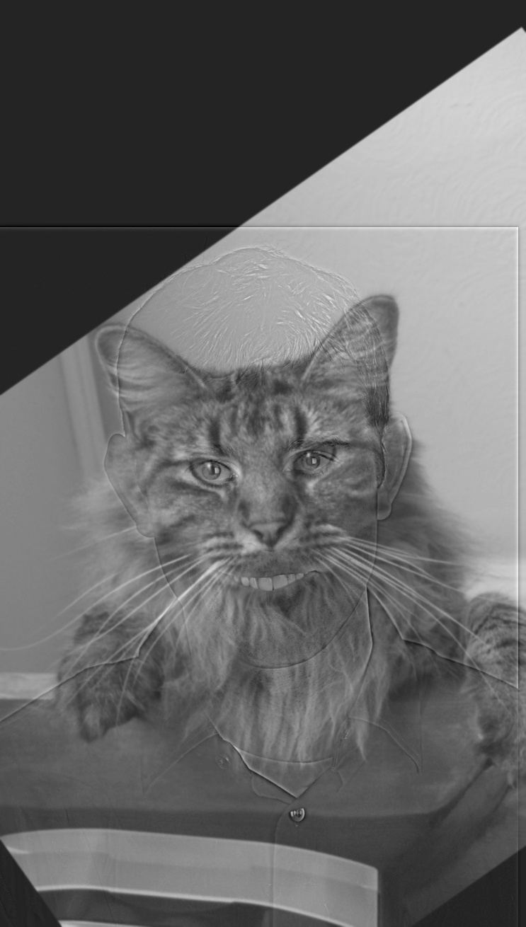
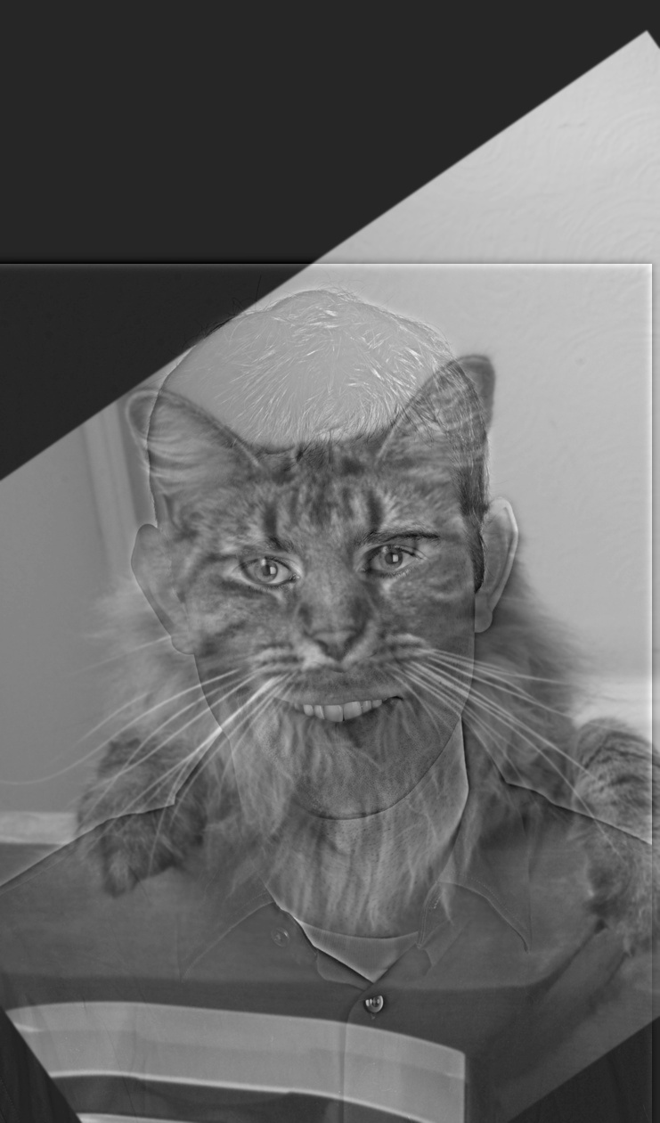
This procedure exploits how human vision works, in which we overlay high and low frequencies of two images over each other to create a hybrid. A low frequency image is created by applying a Gaussian filter, while a high frequency image is created by subtracting its Gaussian filter. This allows the image to feel “merged” in a way, but viewing it from far or near has a large impact on what kind of exact thing you see. When applicable, the centers of the eyes are used as the anchors for alignment purposes. The weights, denoted by Σ, affect how pervasive each image will be in the final result. The image above, which looks the best in my personal opinion, was achieved with Σ=1 on Nutmeg and Σ=6 on Derek, but other values for Derek’s image are shown below:
Derek Σ=2 | Derek Σ=4 | Derek Σ=6 |
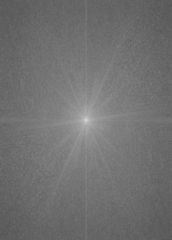
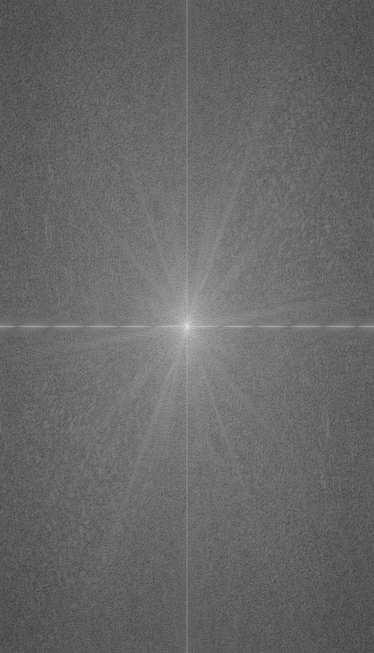
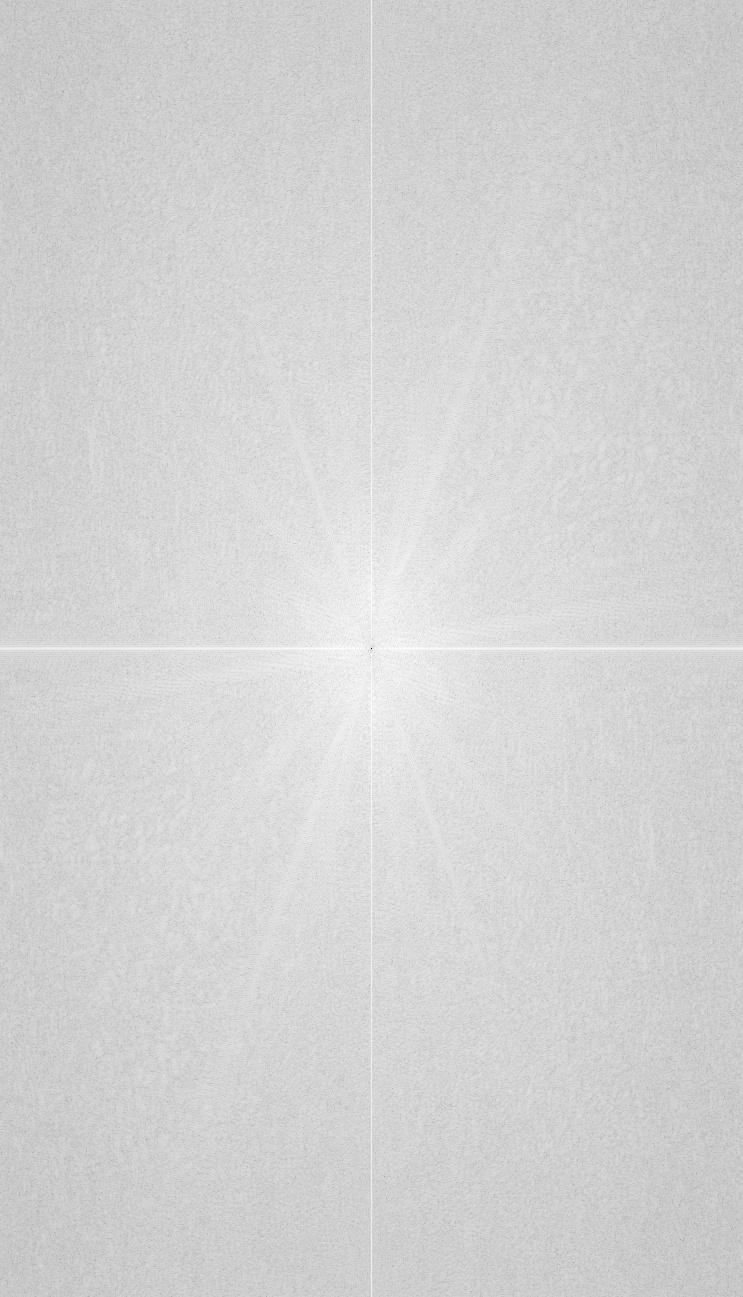
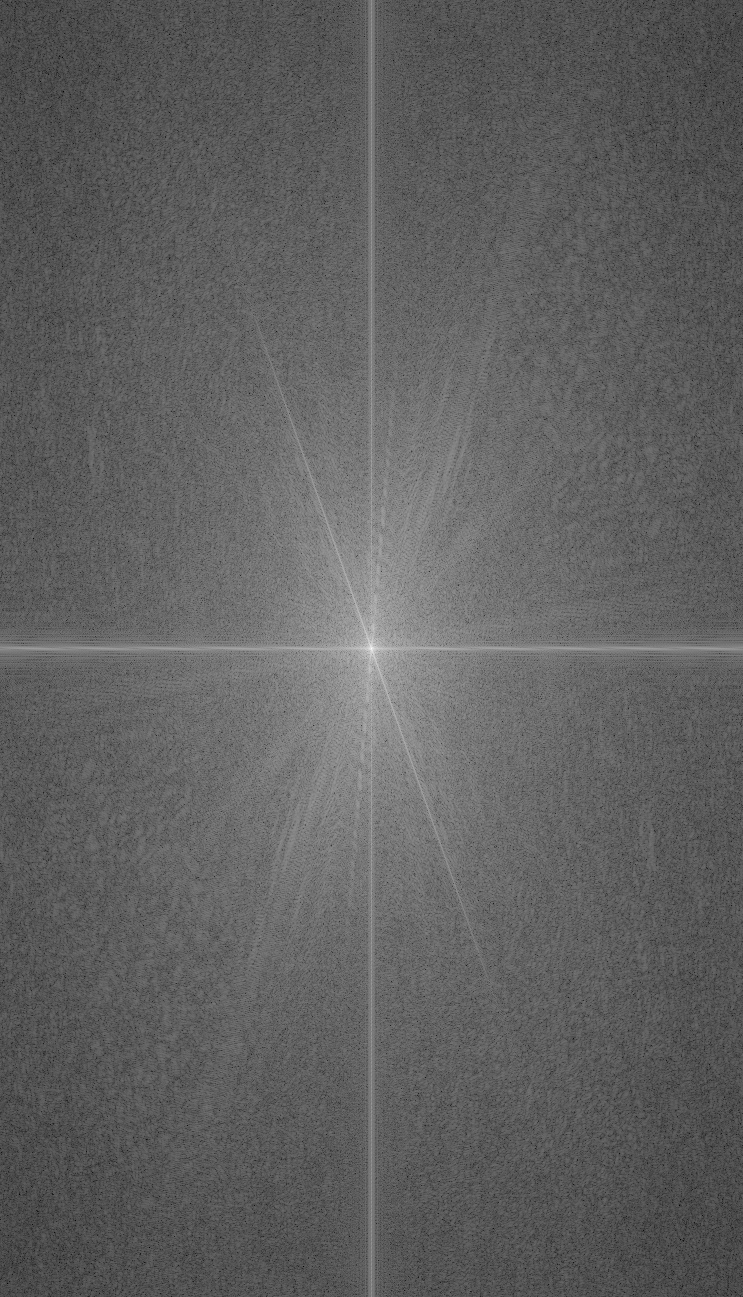
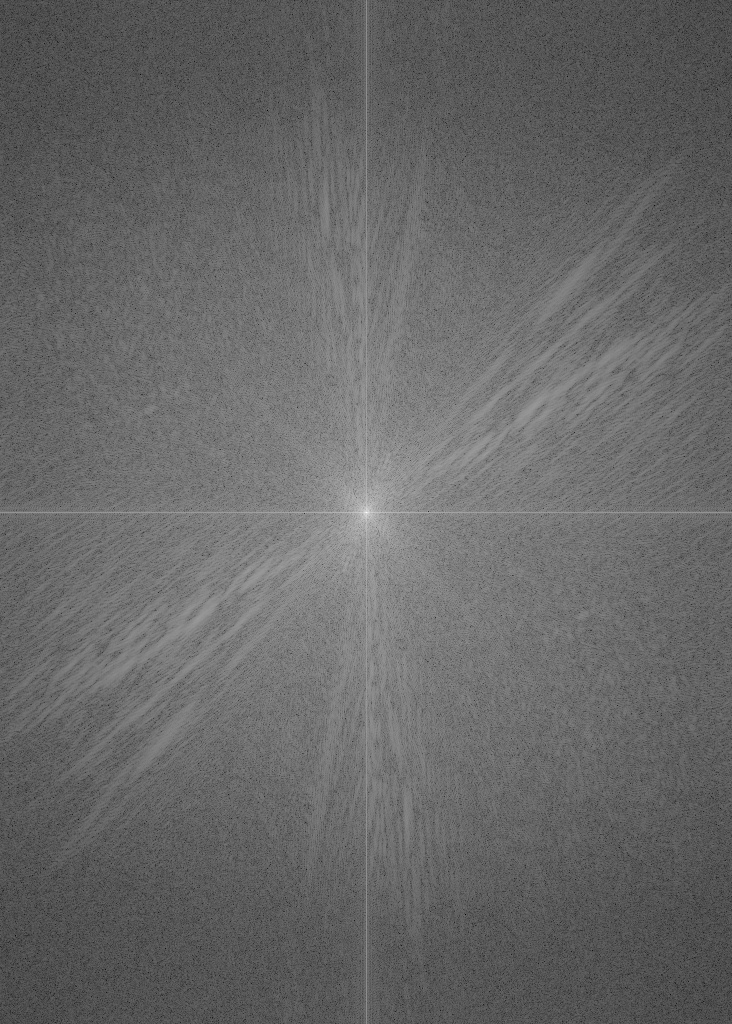
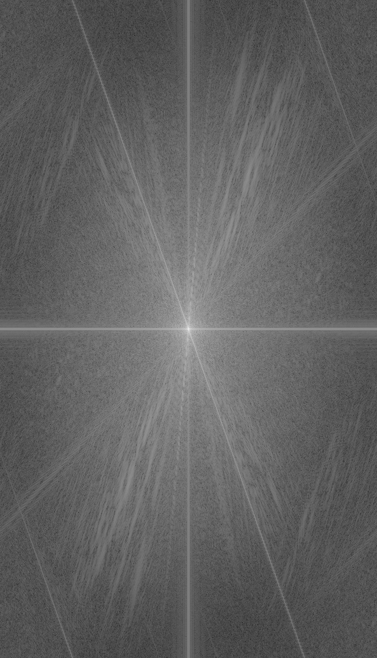
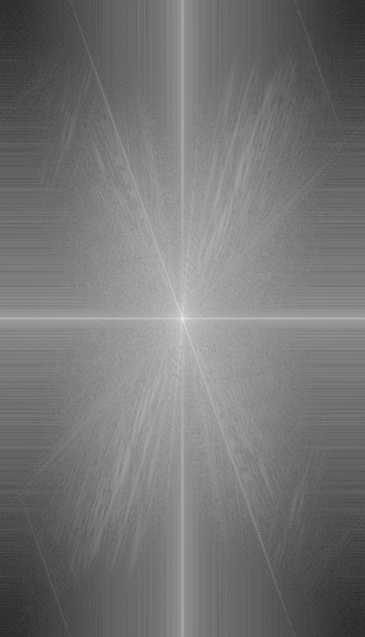
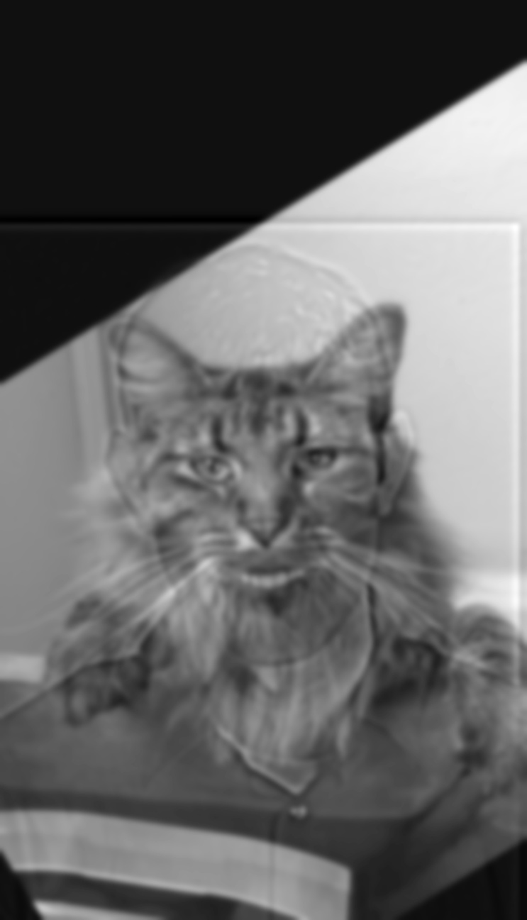
Shown below are the FFT results of the Dermeg hybridization:
Derek - Original | Derek - Aligned | Derek - Filtered | Dermeg - Hybrid Result |
Nutmeg - Original | Nutmeg - Aligned | Nutmeg - Filtered |
The results of some other hybridizations can be seen below:
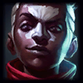
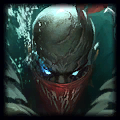
Ekko (Σ=3) | Pyke (Σ=0.3) | Eke |
Since both images begin with identical aspect ratios, alignment gets a little wonky. Still, both characters have eyes, so most of the facial features end up more-or-less lining up and being properly observable. Ekko’s pupils are mostly lost within Pyke’s glowing eyes, which looks kinda neat. Interestingly, since once half of Ekko’s face is darkened, half of his mouth concedes the space to Pyke’s neckerchief. Overall, this turned out pretty alright.
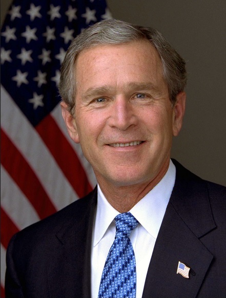
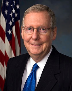
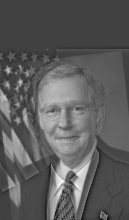
George W. Bush (Σ=5) | Mitch McConnell (Σ=1) | Mirge McUsh |
This pairing was done at personal request of a friend, and turned out pretty well too. Slightly more emphasis had to be put on McConnell than I would’ve liked, but the near-far relationship still exists and Bush can still be identified. McConnell’s glasses actually disappeared, for the most part; you can see them if you’re looking, but otherwise they aren’t very noticeable. Their facial features lined up, despite them facing slightly different directions, and overall, while I don’t think the piece itself looks the best, I think this result best showcases how exactly perception can change from near or far in this kind of hybridization.
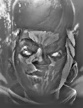
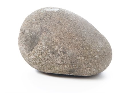
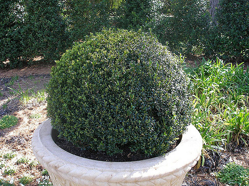
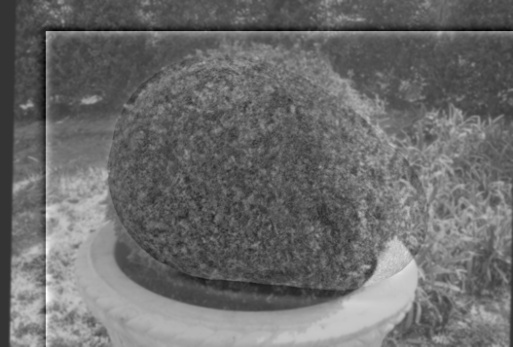
Rock (Σ=5) | Hedge (Σ=1) | Heck |
This one turned out… well, not so great. It works to a certain degree, as the natural texture of the rock actually works surprisingly well with that of the hedge, but in the end a rock is a rock, a hedge is a hedge, and it’s only sort of there. The outline helps, and the rock can be considered identifiable, but without the help of facial features and precognitions about what things are supposed to look like (which help the people examples a lot), this one sort of falls flat.
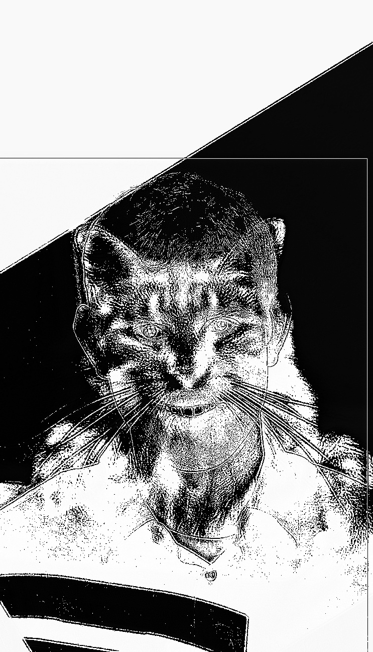
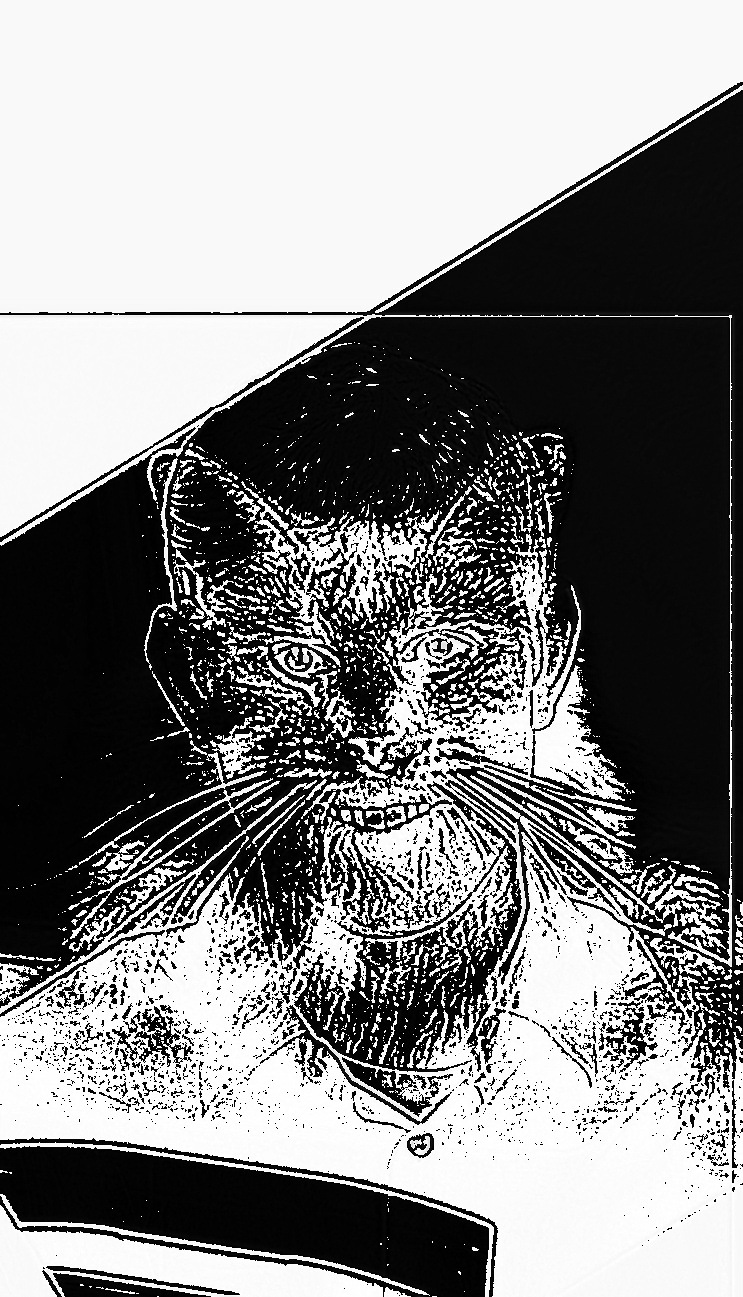
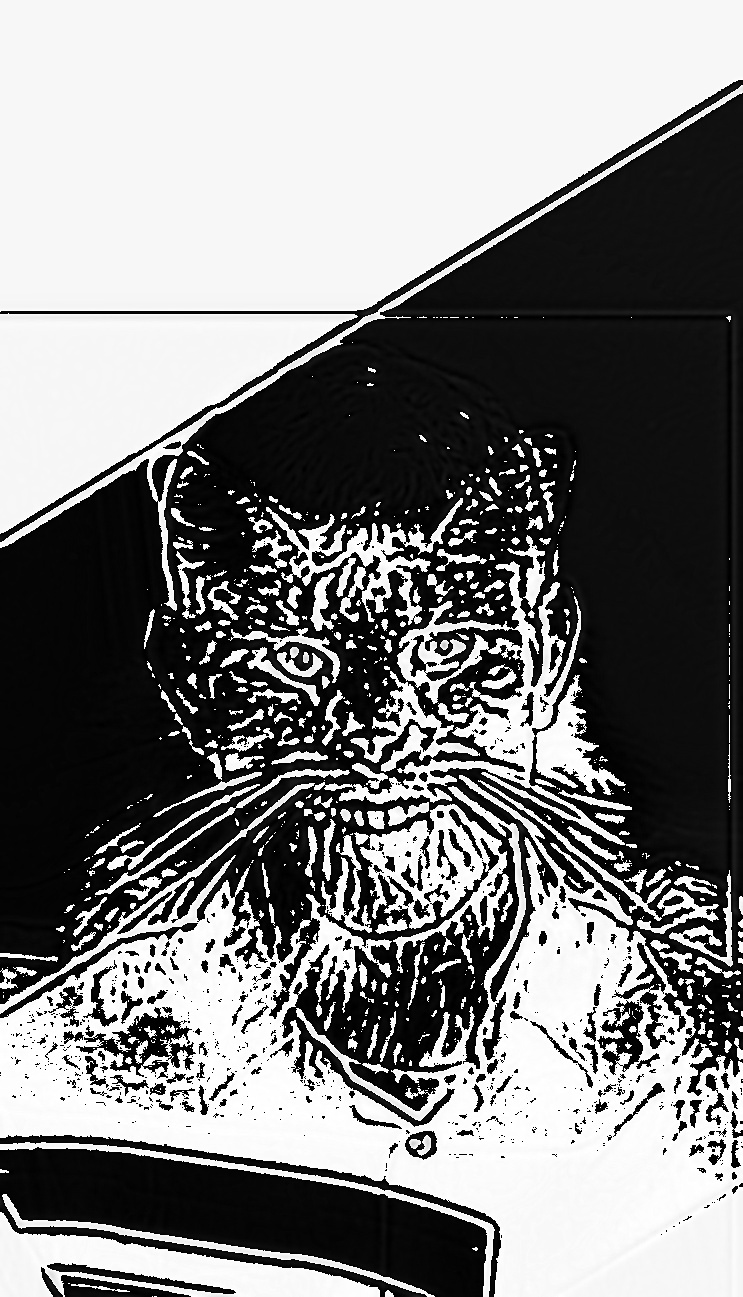
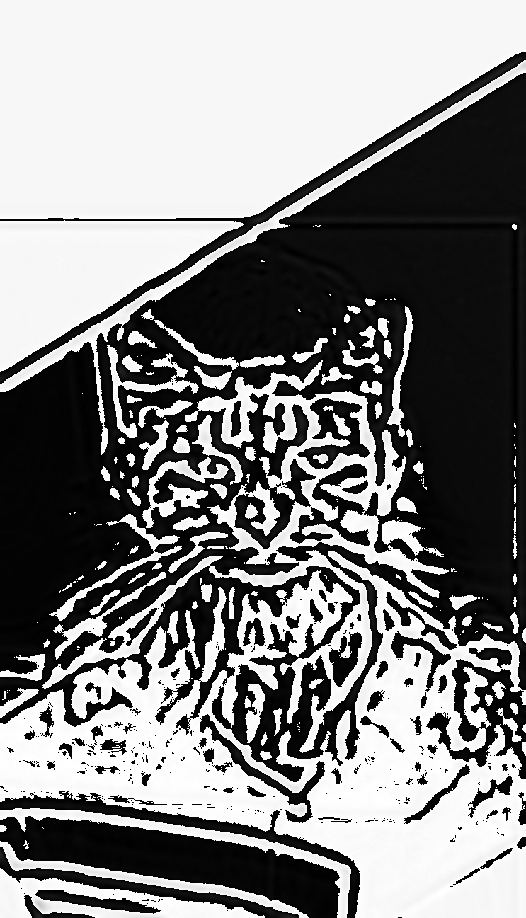
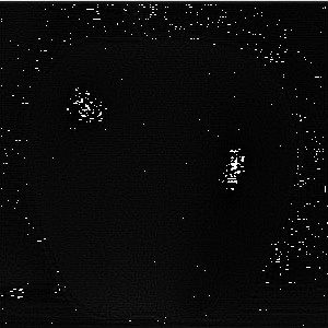
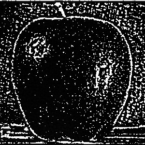
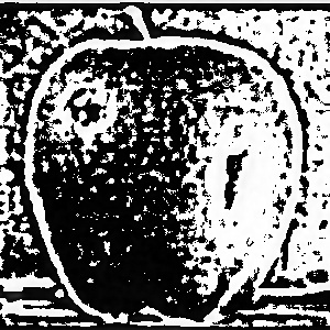
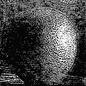
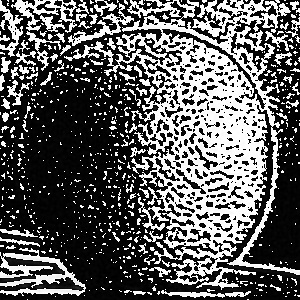
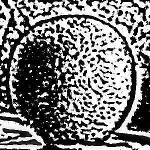
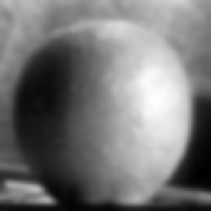
1.3 Gaussian and Laplacian Stacks
Here, we construct Gaussian and Laplacian Stacks, the former heavily relying on the latter. Gaussian Stacks consist of repeated Gaussian filtering on the image, while Laplacian Stacks are represented by the differences between each Gaussian level. For example, the 2nd Laplacian Level is Gaussian Level 1 minus Gaussian Level 2. Our base cases are Level 1 and 8 of the Laplacian Stack, which are just a black image and the 8th Gaussian Stack, respectively. The black image is intuitive since the first level cannot differ from the original, and the last level allows us to reconstruct the image. The results of a few examples are shown below:
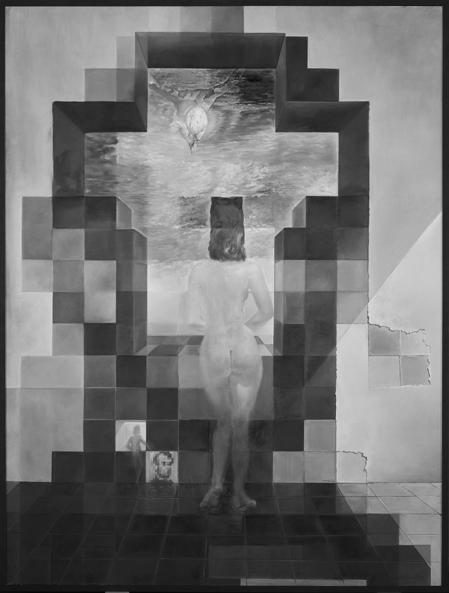
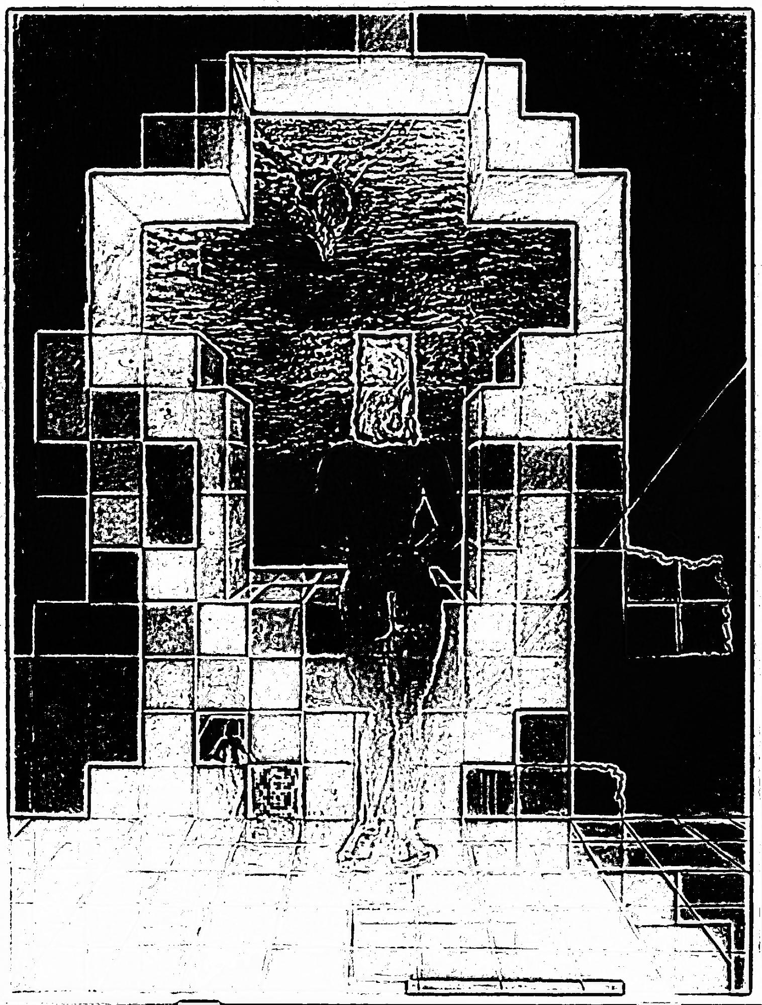
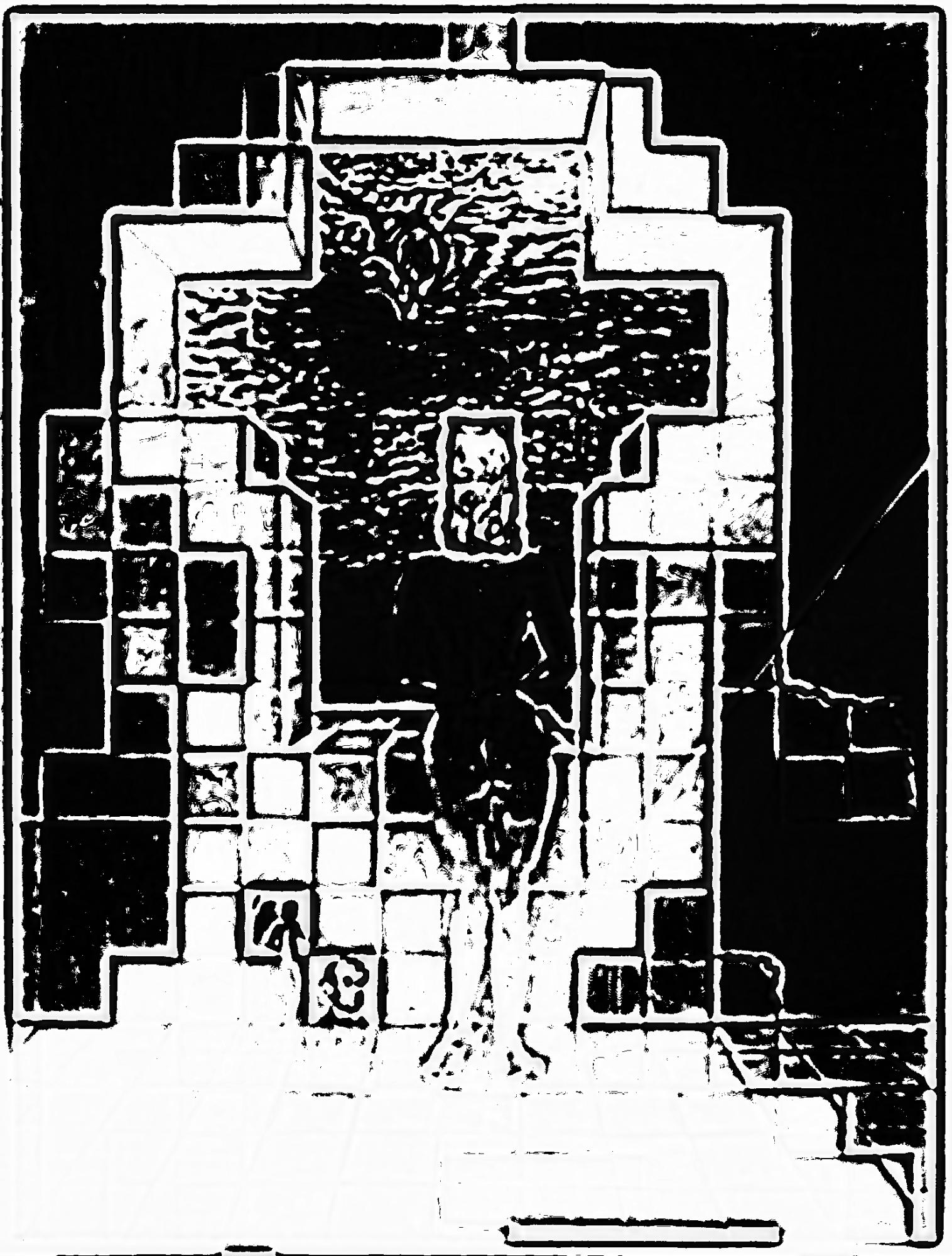
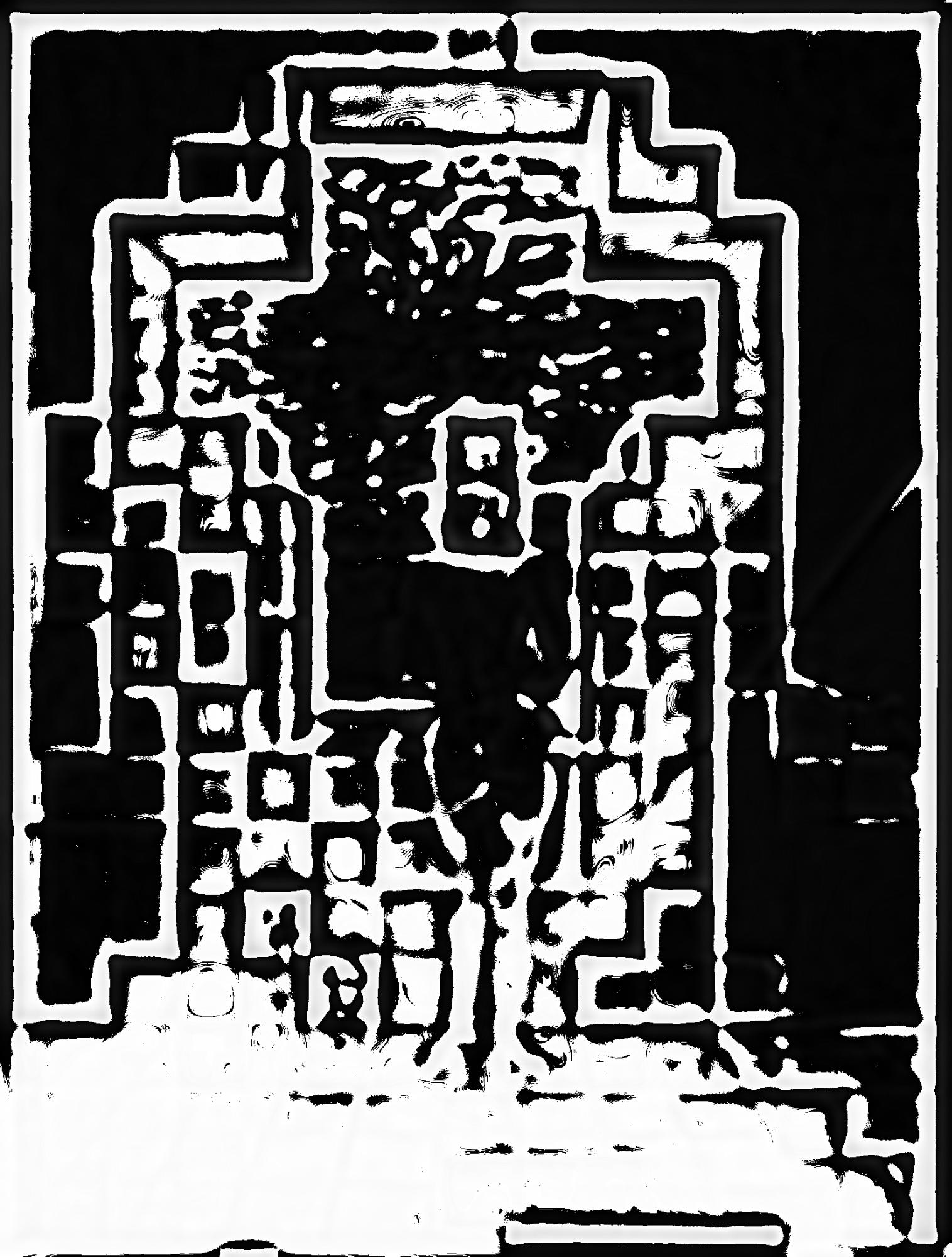
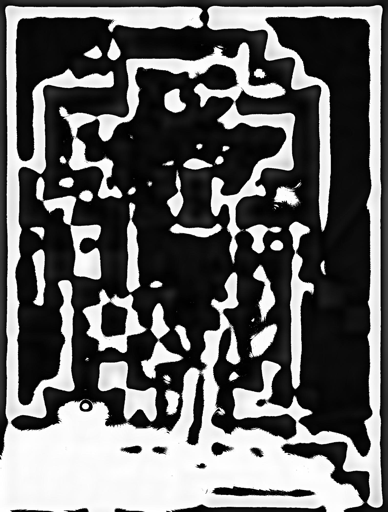
Gala Contemplating the Mediterranean Sea which at Twenty Meters Becomes the Portrait of Abraham Lincoln-Homage to Rothko by Salvador Dali
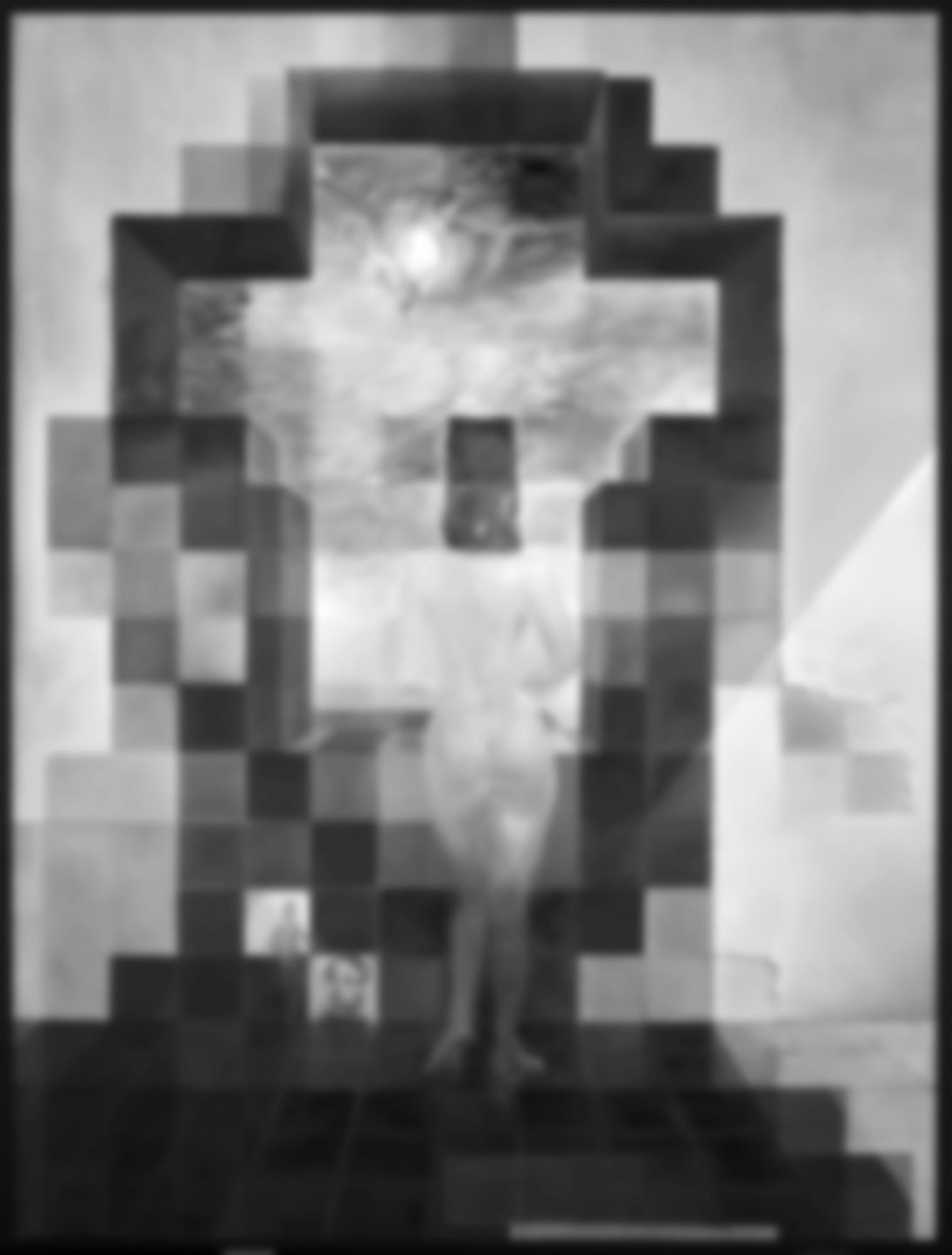
Gaussian:
Level 1 | Level 2 | Level 3 | Level 4 |
Level 5 | Level 6 | Level 7 | Level 8 |
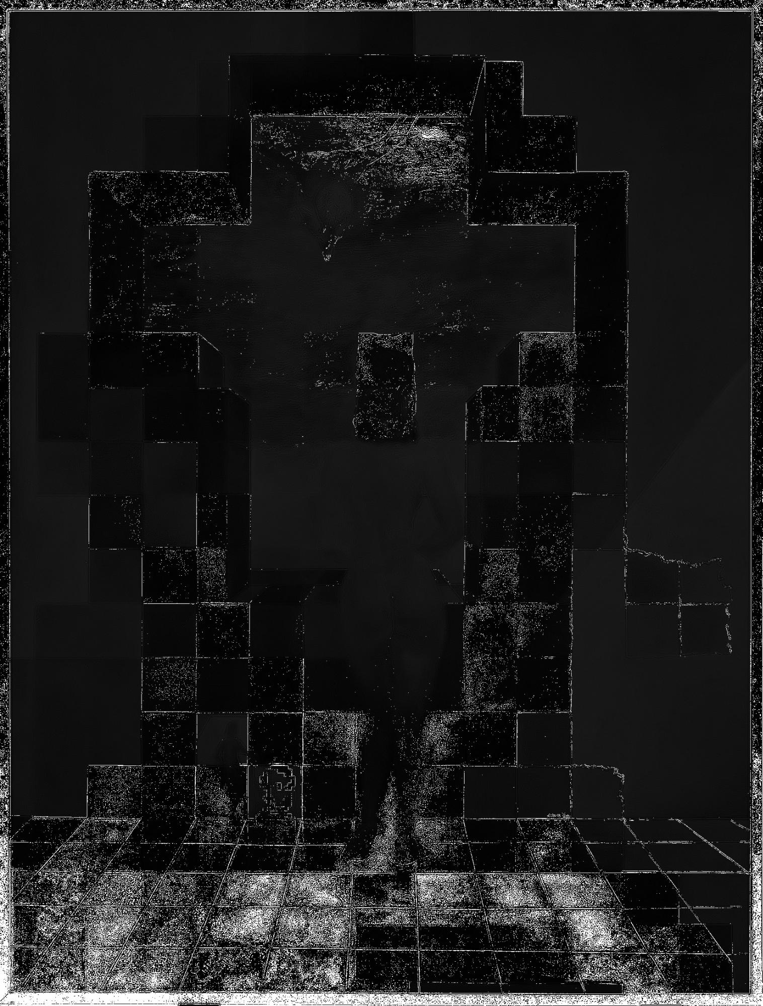
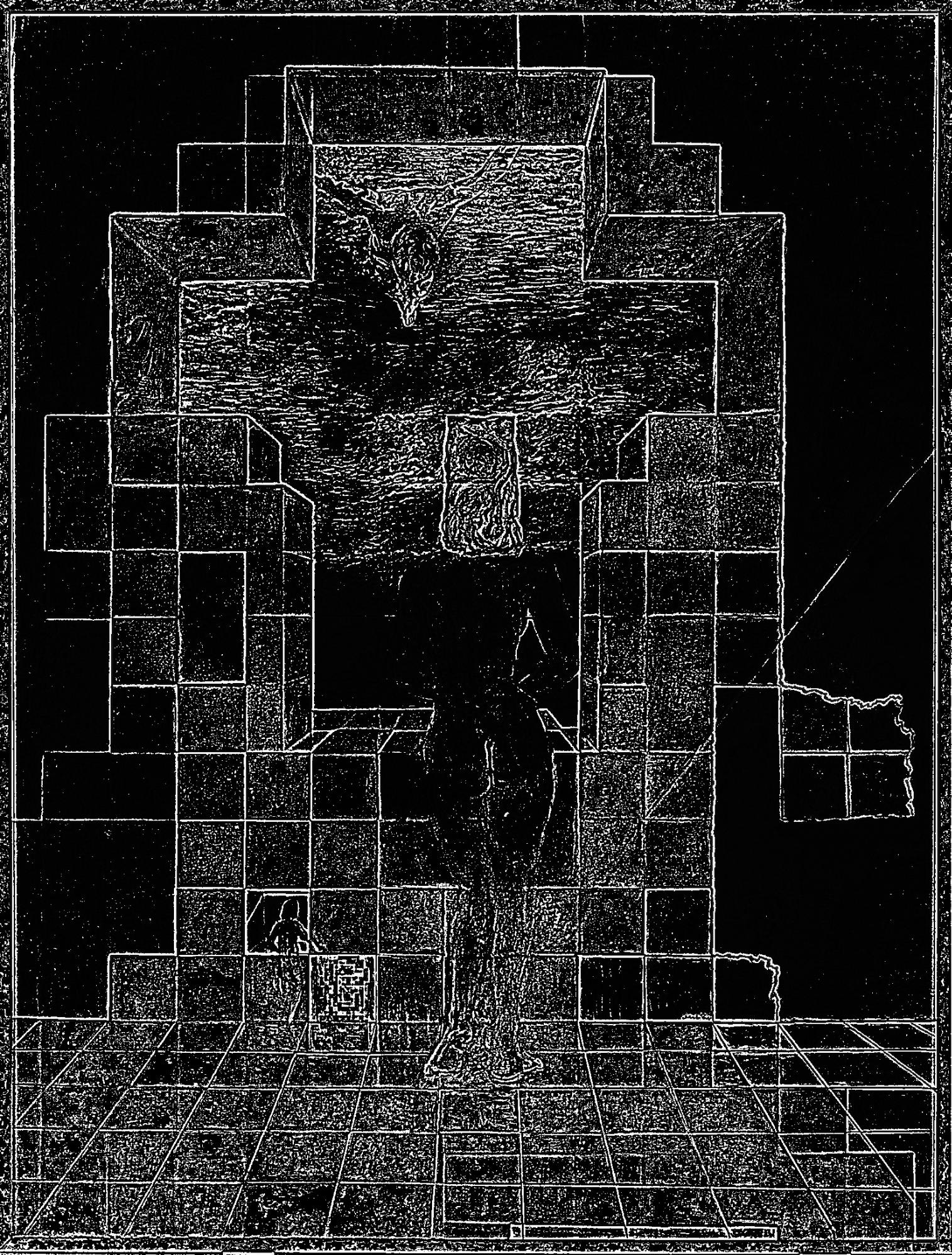
Laplacian:
Level 1 | Level 2 | Level 3 | Level 4 |
Level 5 | Level 6 | Level 7 | Level 8 |
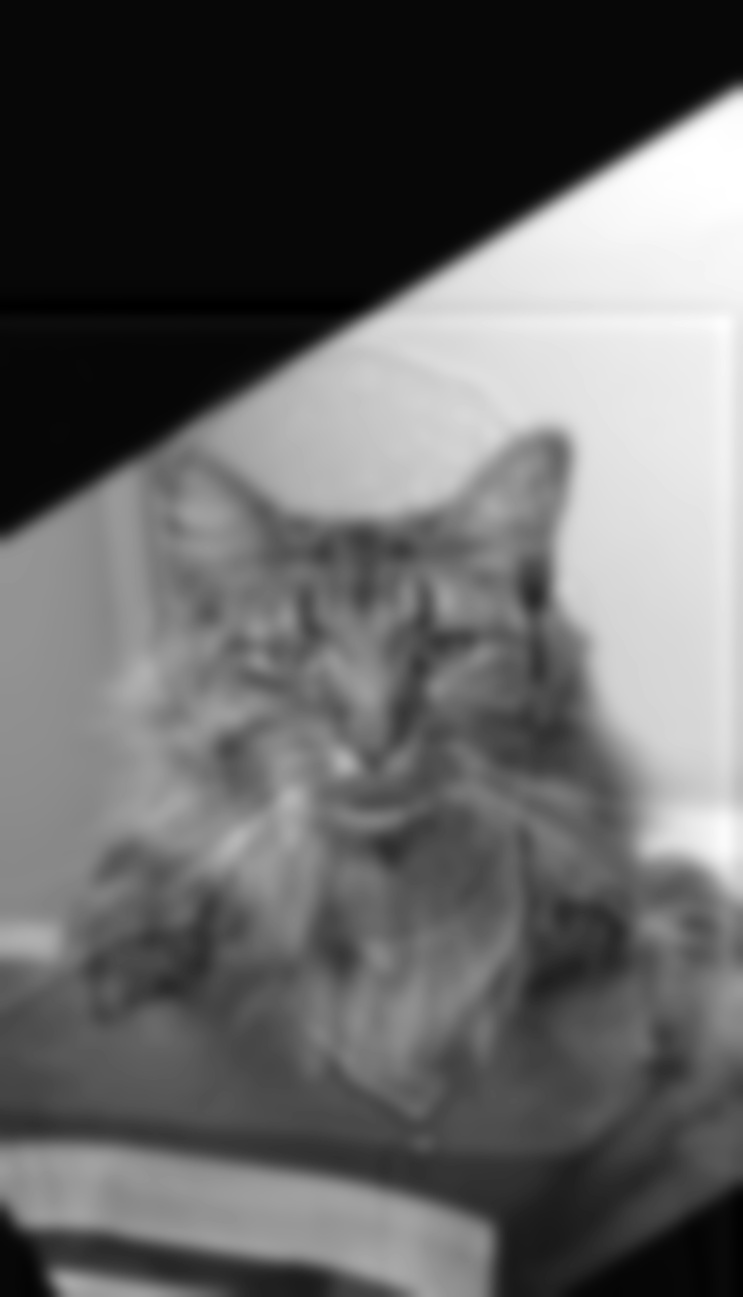
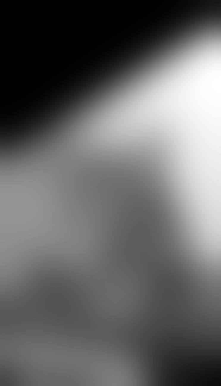
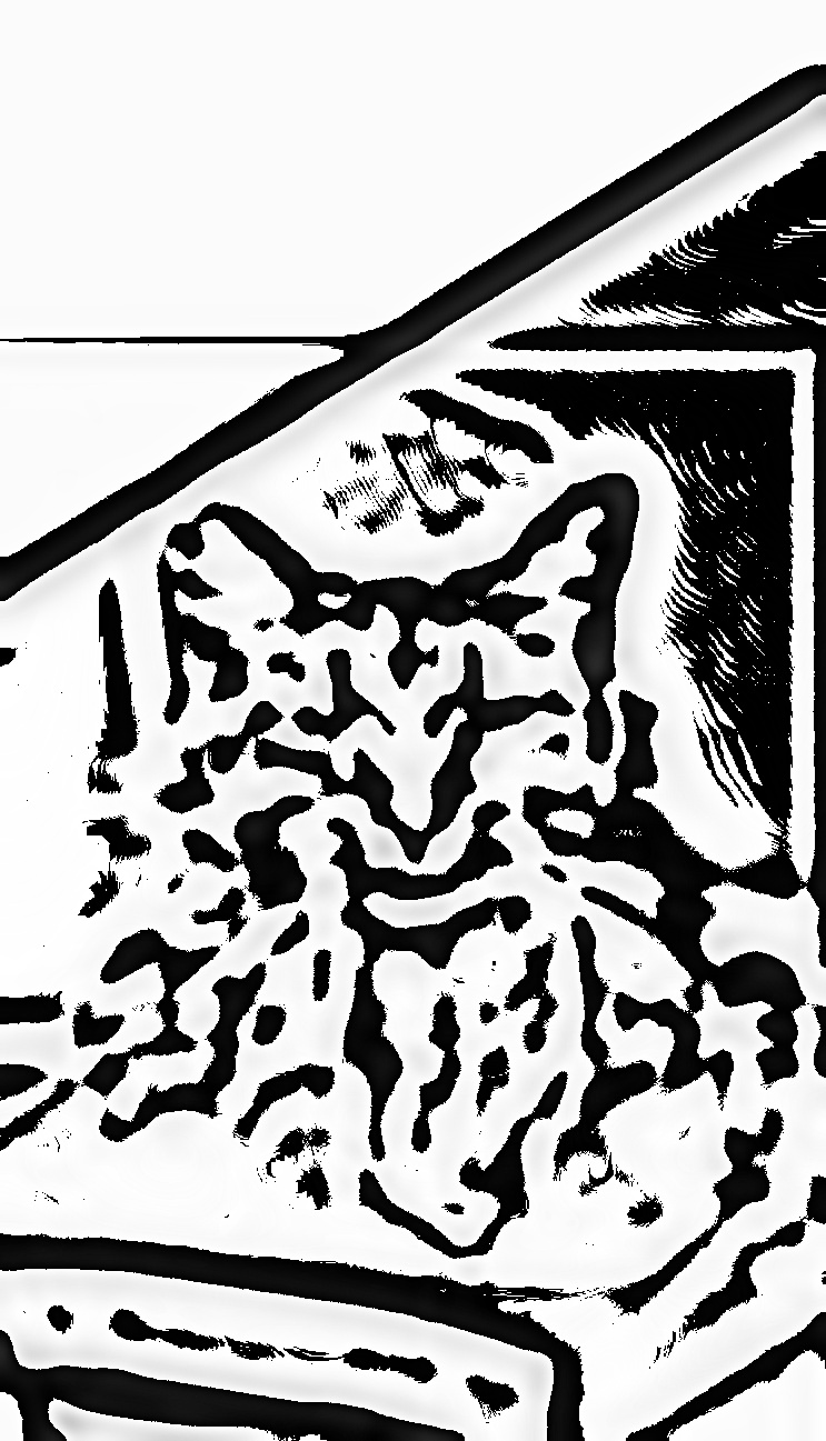
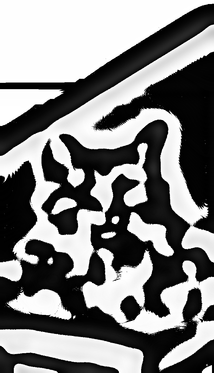
Dermeg Hybridization
Gaussian:
Level 1 | Level 2 | Level 3 | Level 4 |
Level 5 | Level 6 | Level 7 | Level 8 |
Laplacian:
Level 1 | Level 2 | Level 3 | Level 4 |
Level 5 | Level 6 | Level 7 | Level 8 |
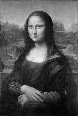
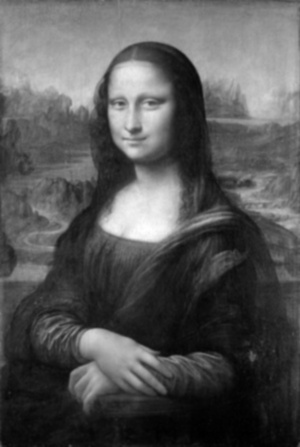
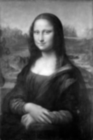
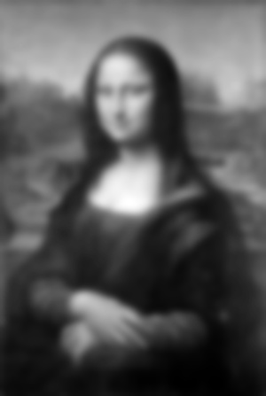
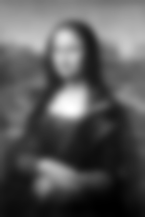
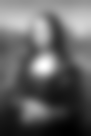
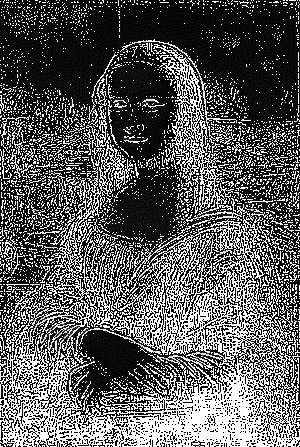
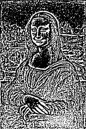
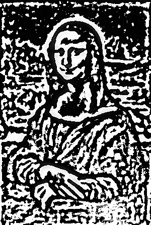
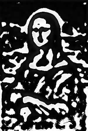
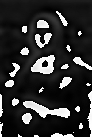
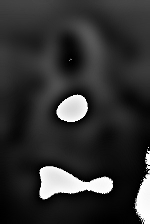
Mona Lisa by Leonardo da Vinci
Gaussian:
Level 1 | Level 2 | Level 3 | Level 4 |
Level 5 | Level 6 | Level 7 | Level 8 |
Laplacian:
Level 1 | Level 2 | Level 3 | Level 4 |
Level 5 | Level 6 | Level 7 | Level 8 |
1.4 Multiresolution Blending
Using the same fundamentals of the stacks, we can then start merging images together more cleanly by breaking them into stacks first. For each level, we create a Laplacian filter for each input image, and an equivalently-leveled Gaussian filter for our appropriate shaping mask. This mask, which consists of only black and white, allows us to control which input appears where.
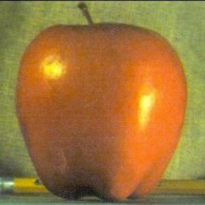
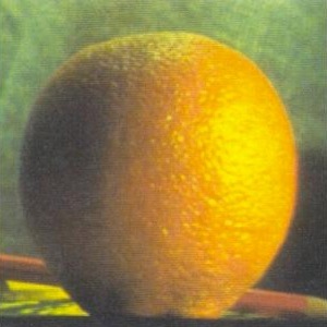
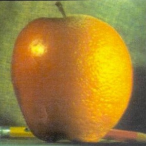
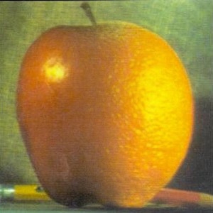
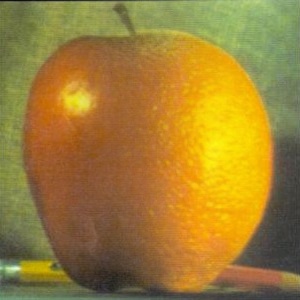
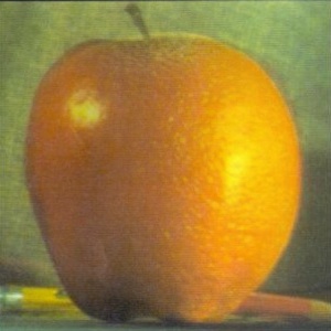
The main variables to be modified are the number of layers, as well as the appropriate Sigma for each input. The more layers there are, the larger the blurred seam region is, which can either be good or bad depending on context. Below, you can see the Orapple merge at multiple layer levels, but eventually the stem of the apple becomes ghostly and the additional layers could be considered a detriment.
Apple (Σ=0.0005) | Mask | Orange (Σ=0.05) |
4 Layers | 8 Layers | 16 Layers | 32 Layers | 64 Layers |
For context, here are the some of the Laplacians and Gaussians:
A few more examples are below:
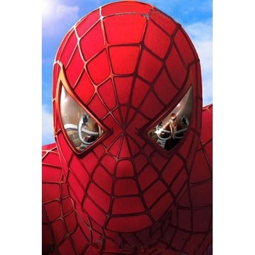
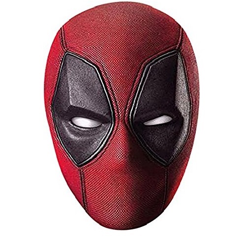
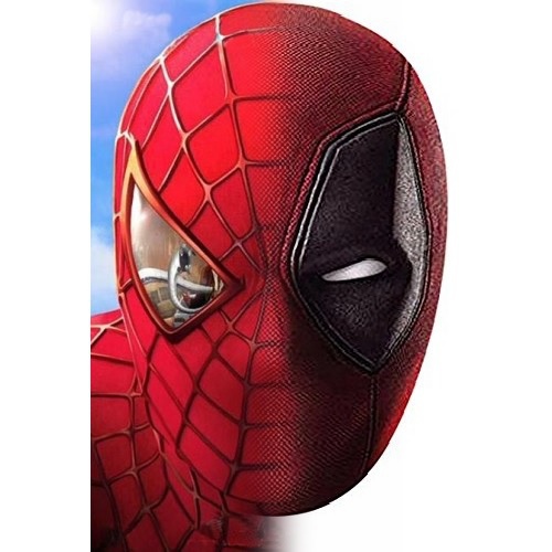
Spiderman (Σ=0.0005) | Mask | Deadpool (Σ=0.001) | Deadman |
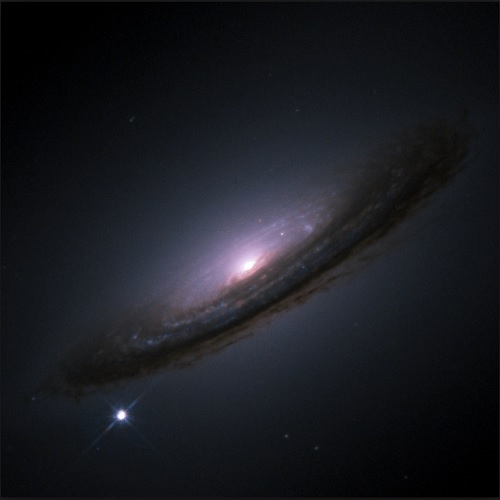
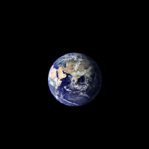
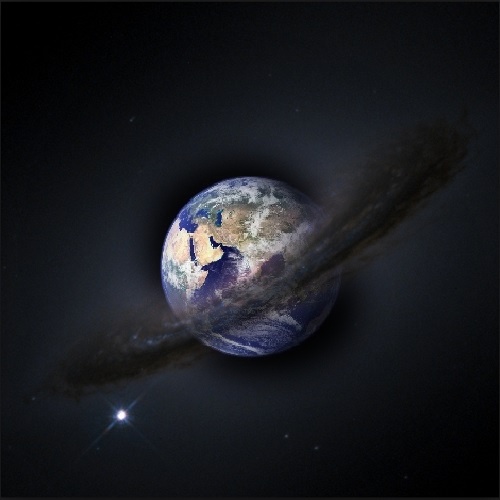
Supernova (Σ=0.0005) | Mask | Earth (Σ=0.001) | A Big Mistake |
2.1 Toy Problem
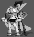
As an intro to the following, more complicated Poisson Blending problem, we begin with a smaller, toy problem, where we break down a picture of Buzz and Woody, recreating it using its gradients. We construct a basic linear least-squares system (v = Ab), where we match the top left pixel of input and output images to calibrate. We attempt to optimize the three following principles:
where v denotes the output and s denotes the source. By doing so, we are able to achieve the following, where the goal is for the reconstructed version to look as close to the input as possible.
Input | Reconstructed |
We then expand on this principle as we move forward to the finale of the project:
2.2 Poisson Blending
The meat of the project culminates here: poisson blending. With this technique, we can blend more particularly than with multiresolution blending. The largest advantage of this method is its cleaner gradients, which lets us paste other objects into images without sharp, obvious edges. I began with the masking tool starter code graciously provided by Nikhil Shinde on Piazza to create the masks. Ultimately, the inputs necessary for my algorithm were a source image, a target image, and the mask (made by the tool personally, but any mask works), all of which must be the same resolution. Only a single mask is used for simplicity, so the source image should just be moved around ahead of time to match a single mask; I tried having better mask conversion using the two given by the starter code, but the algorithm became much cleaner with only three inputs. Any discrepancies caused by the smaller input count can be resolved via prior cropping and resizing, which is easy to do in basic programs like Paint and Photoshop.
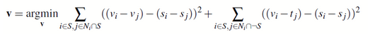
To start, I parse the mask, recording all pixels are on the inside of the mask, and any that are on the border have which sides they border it on recorded. This is the most essential aspect of the later gradient creation, as it lets us detect what must be blurred. Moving forward, we use similar logic as before, relying on least-squares solutions; however, this time, we build A as a sparse matrix, as this greatly reduces runtime for our now-larger inputs. Anything not in the mask or near its edge is irrelevant for this transformation, we everything not being blended will be left the same as how target started by default. We then create the system’s vector b with the given Poisson equation,
,
and solve each channel separately to maintain color (these are recorded as three separate columns of b, which is only solved one column at a time). Finally, we clip these colors back into a resulting image (limiting to 0-255 just in case), at which point we are done. We can see the results for multiple examples below:
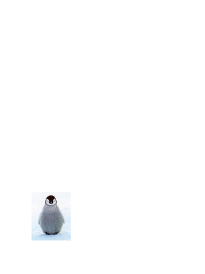
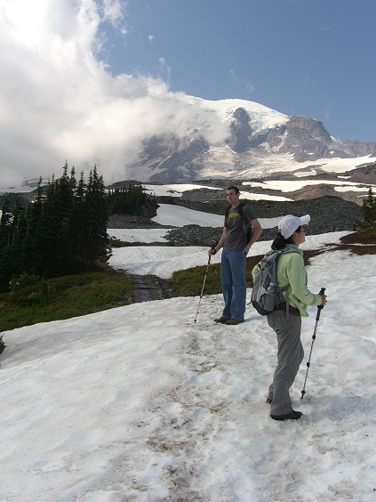
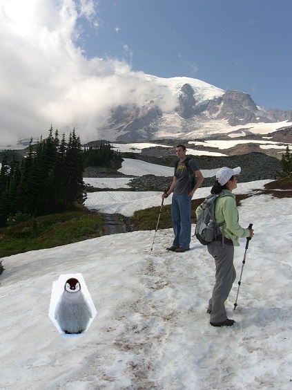
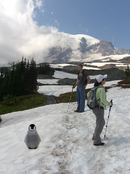
Penguin Chick | Snowy Hillside | Naive Paste | Poisson Blend |
This first one, which uses the given images, turned out really well! The perspective doesn’t exactly make sense with why a penguin would be stand like that in that position, but overall the gradient came out almost seamlessly and I’m very proud of how it turned out.
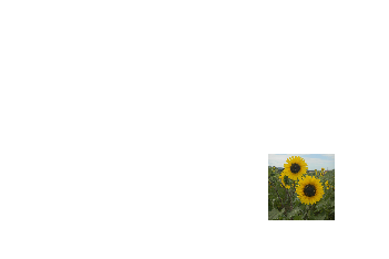
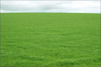
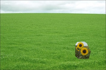
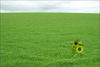
Sunflowers | Field | Naive Paste | Poisson Blend |
Another fairly basic one, we put sunflowers in a field. Since the surroundings of the sunflowers were already green, it seemed like this would go well, but there’s actually sky in the background, so the gradient gets very confused. Ultimately, this was a failure case, as we basically ended up with half-green sunflowers melting into a field with a weird void behind them. This showcases one of the flaws with my algorithm, which is that it greatly dislikes rapid color variance when blending, like grass vs sky in the sunflower picture. It’s still way better than naive, though, and without the sky would probably look pretty good.
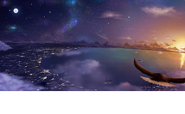
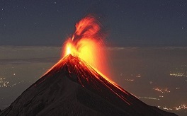
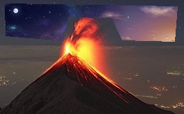
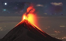
Starlit Sky | Erupting Volcano | Naive Paste | Poisson Blend |
This one is very aesthetically pleasing, it does have its flaws, namely because it is trying to blend in a background rather than an object. While maybe not immediately obvious, it is very easy to see where the mask was cut (particularly around the eruption, but also the picture edges), since there isn’t a way to create generous mask margins since the sky itself has no border in the original image. It still looks nice, though, and even with the current algorithm could probably look even better with some tweaking!
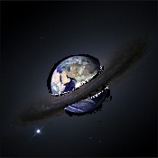
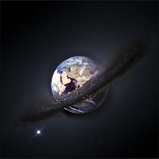
Earth | Supernova | Naive Paste | Poisson Blend |
I think that the Poisson Blend here looks vastly better than the stack version, mostly because the ring around the earth is able to completely conceal the planet’s body, as opposed to the transparency noticeable in part 1.4. It is a little strange how emphasized the ocean has become in the Poisson version (the glaring purple area), which may be the result of it being blended with the purple star core in the supernova image. The earth also doesn’t appear to glow as much black light as it did previously, but that’s almost certainly due to how the mask is set up and could be remedied (or added back in) with some adjustments. Given the complex nature of this blending, I think it’s intuitive that this version came out better.