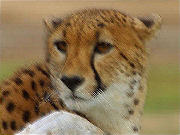
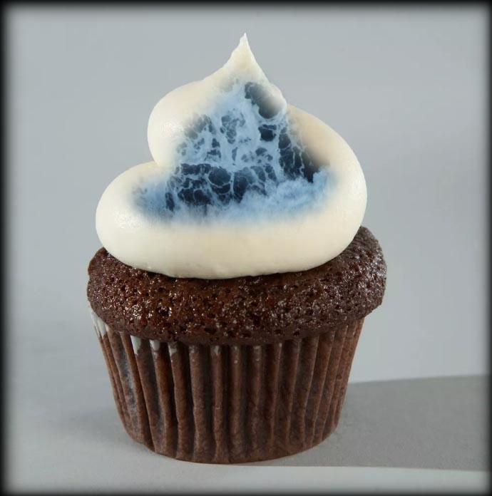
The unsharp mask filter involves first using a Gaussian kernel and convulving it over the blurry image. This resulting blurred image serves as mask to be combiend with the original image, which ultimately sharpens the image. For the warmup, I used a blurry picture of a cheetah and played around with the alpha value. I saw that as my alpha value increased, the resulting picture appeared sharper. I settled on an alpha level of around for my final image.
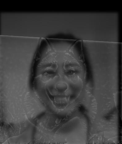
The approach for making the hybrid images plays with high and low frequencies. As explained in the paper by
Olivia, Torralby, and Schyns, the hybrid images are static but appear to change depending on the viewing distance.
This effect is caused by using different frequencies for different images and blending them together. As a result,
the image whose lower frequency is used is clearer when viewed from afar, while the image with a higher frequency
can be more clearly seen from close up.
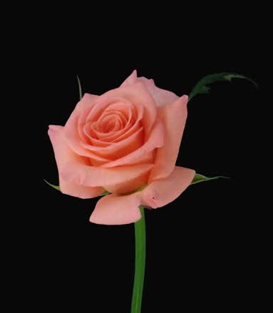
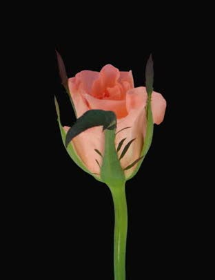
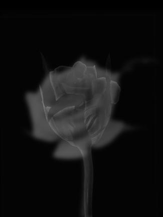
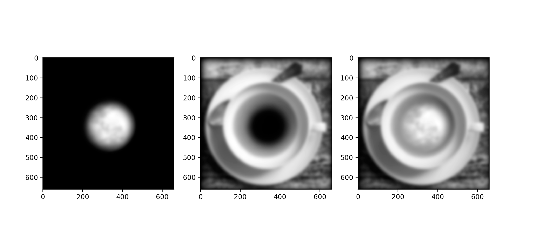
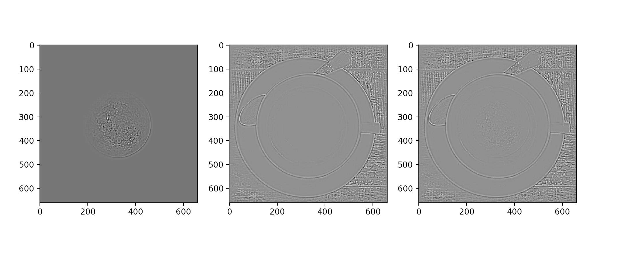
To isolate the high and low frequencies for the images, the same technique as Part 1.1 was utilized. Applying the Gaussian
filter results in an image with low frequencies, while subtracting the convolution of the filter and an image results in
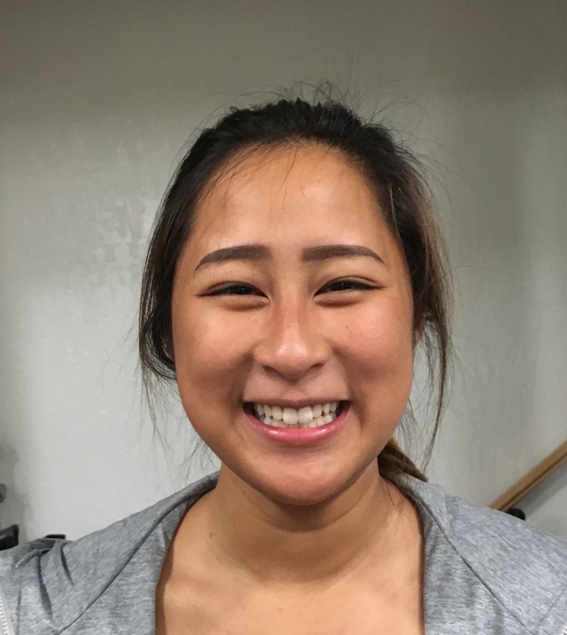
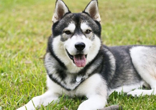
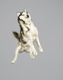
a high frequency image. The image of the flower opening was the most effective for me, while the image with the husky
in the bottom row did not work as well. As you can see in the hybrid image, the strong contrast
of the husky's features resulted in its outline rather than the image itself being clear at low frequency.

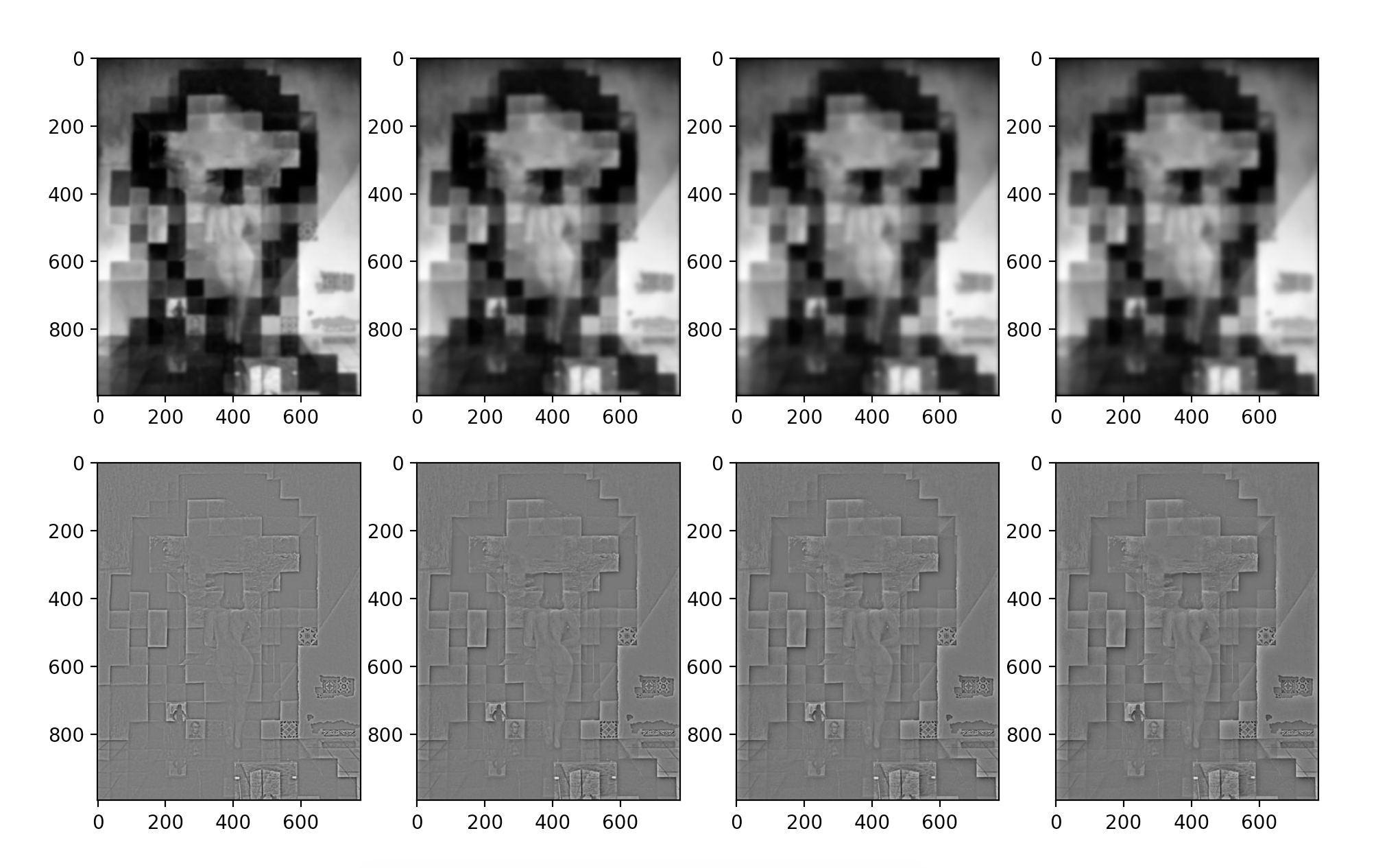
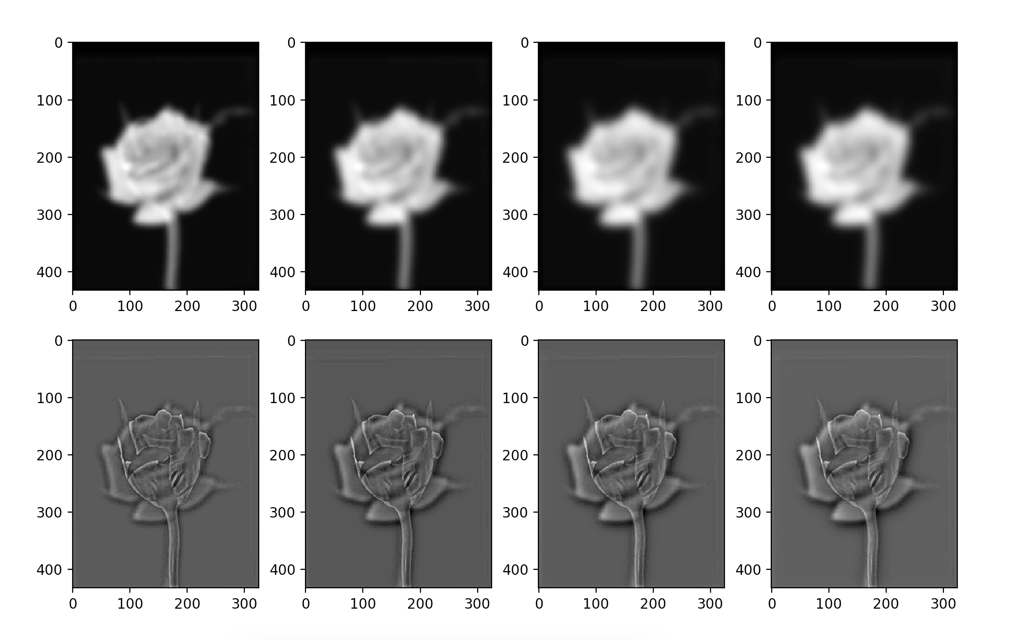
The Gaussian and Laplacian stacks show what aspects of the image are easily viewed at each frequency. The Gaussian stacks increase the "blurriness" of the image, or low frequencies of the image, while the Laplacian stacks increase the "sharpness", or high frequencies. The stacks differ from pyramids in that they do not downsample, and instead repeatedly apply the Gaussian filter (or subtract the application of the Gaussian filter) to an image to demonstrate the different frequencies.
To effectively blend together the images, the mask and the input images are both blurred with the Faussian
filter to make the transition between images of different resolutions more seamless. We employ the Gaussian pyramid
from the previous part in order make the edge of the mask less sharp and, consequently, smooth out the
final image.
Initially, this was applied to grayscale images, but I then applied the same technique to the three color channels
to see how the image would look in color after being blended together. Because color is another difference between
the two images being blended together, I found that I had to increase the sigma of the Gaussian filter applied
to my masks in order to make the colored images smooth in transition.
The challenging part of the Toy Problem was deciphering how to convert the constraints to code. After drawing it out on paper, it was easier to visualize how the matrices should be filled out. Essentially, the A matrix is comprised of 0, 1, or -1. The 1 and -1 corresponds to specific v values that equate to a gradient value which is placed in the b vector. Since the image being reconstructed was fairly small, I could get away with not using the csr_matrix function. The image was able to be reconstructed in about 4 minutes of running time.

This section took me by far the longest out of the other parts of the project. I struggled a lot with figuring out how the second constraint, the border constraint, fit in with the existing code for part 2.1. After realizing that it was simply some additional rows in A and corresponding target pixel values in vector b, I spent the rest of the time debugging some mistakes in border indices and array dimensions before successfully blending the penguin into the snow by the hikers.
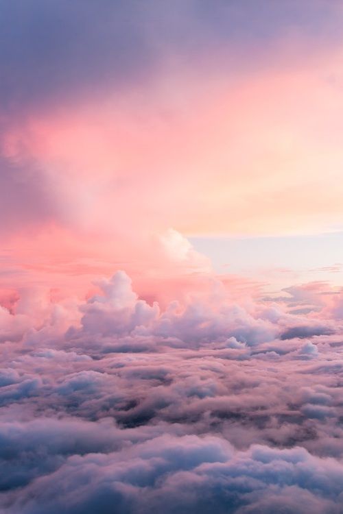
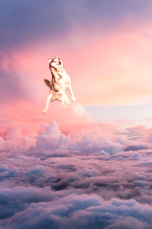
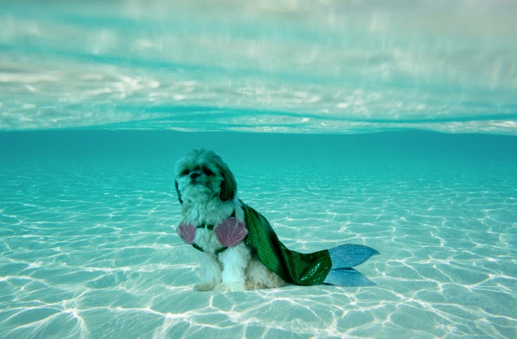
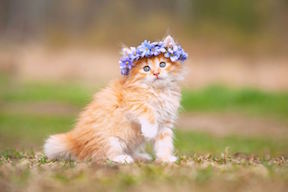
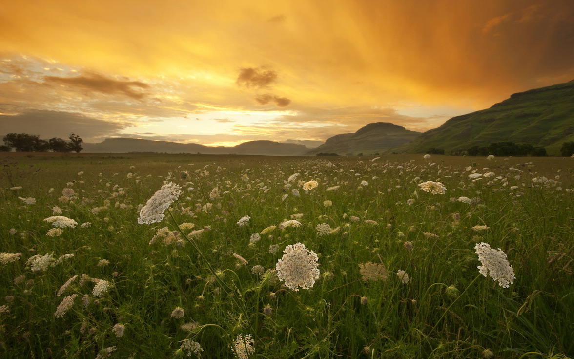
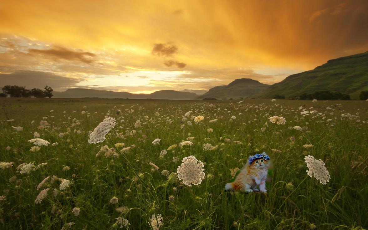
The images in the first row resulted in the most successful blend. I believe this is due to the husky image having a plain, gray background, so the lack of interference with calculating the gradient and the close cropping to the husky resulted in it blending pretty seamlessly with the sky. On the other hand, the image with the cat in the meadow did not work as well. This is due to the background of the target image as well as the source image being too detailed, so the gradient reconstruction was a bit more difficult and less precise. With source images where the background doesn't seem too similar in pattern to the target background, the blending does not look as smooth.


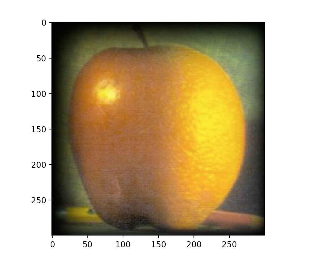
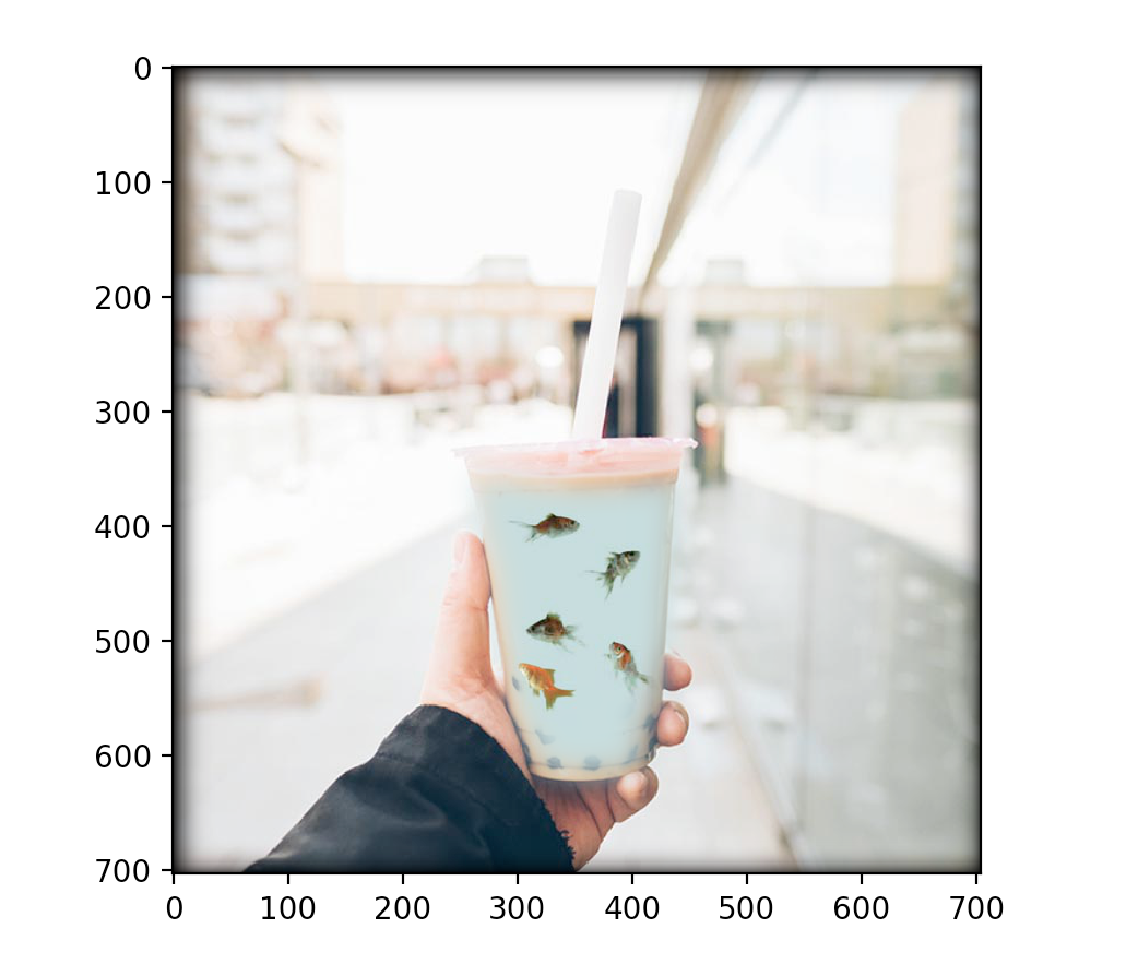
The Poisson blending (last image in the row above) worked better because to give the illusion of the fish being in the boba, the calculation of the pixel values with gradients is more effective. On the other hand, I believe when you wish to preserve the initial colors of the source image (such as when making the source image appear to be on top of the target background) and the colors differ greatly, the Laplacian blending would be better. It would also be better if the transition between the images is supposed to be gradual, such as blending the orange and the apple.