Project 3 - Fun with Frequencies and Gradients
CS 194-26 Fall 2018
By Tao Ong
Part 1: Frequency Domain
Part 1.1: Warmup (Image Sharpening)
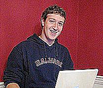
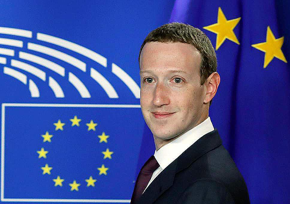
The project's warmup was to pick your favorite image (mine being any picture of the Zuck), and sharpen it using the following technique:
We take some image I and apply a Gaussian (low-pass) filter on it to obtain G,
then we calculate I - G * alpha (where alpha is some constant adjusting the intensity of the sharpening)
to get only the higher frequencies in the original image I.
Finally, we add the result (the higher frequencies) back to image I to sharpen the image.
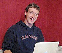
Alpha: 1
Alpha: 5

Alpha: 1
Alpha: 5
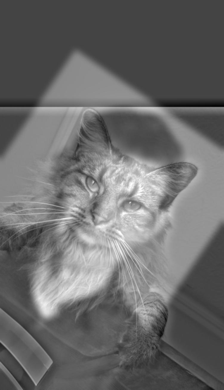
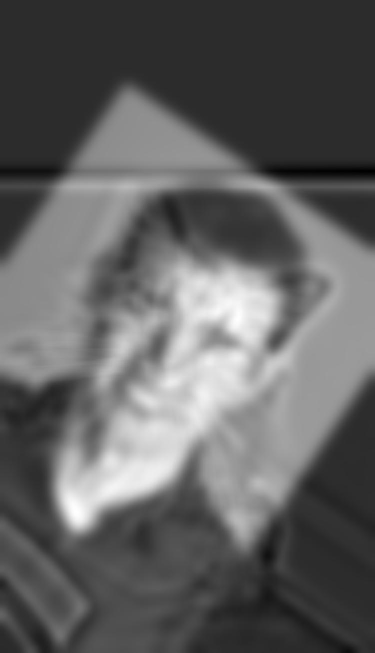
Part 1.2: Hybrid Images
In this section we create hybrid images by combining the high frequency data of one image
with the low frequency data of another image. When we look at this hybrid image from a close
distance, we will see the high frequency data stand out. Similarly, when we view the image
from afar, we will see the low frequency data stand out.
We retrieved the low or high end frequencies of each image by running a either a Gaussian
low-pass or high-pass filter on each image, similar to the method used in part 1.1.
Here are the results on some pairs of images:
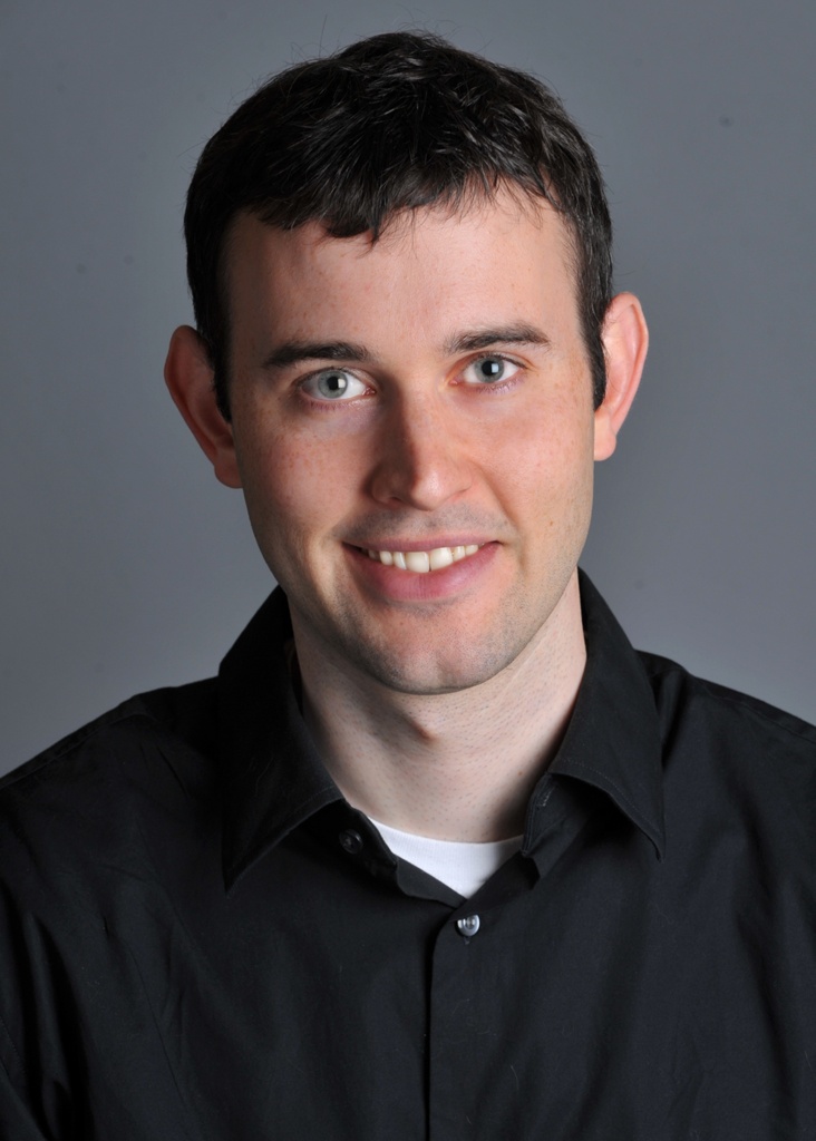
Derek
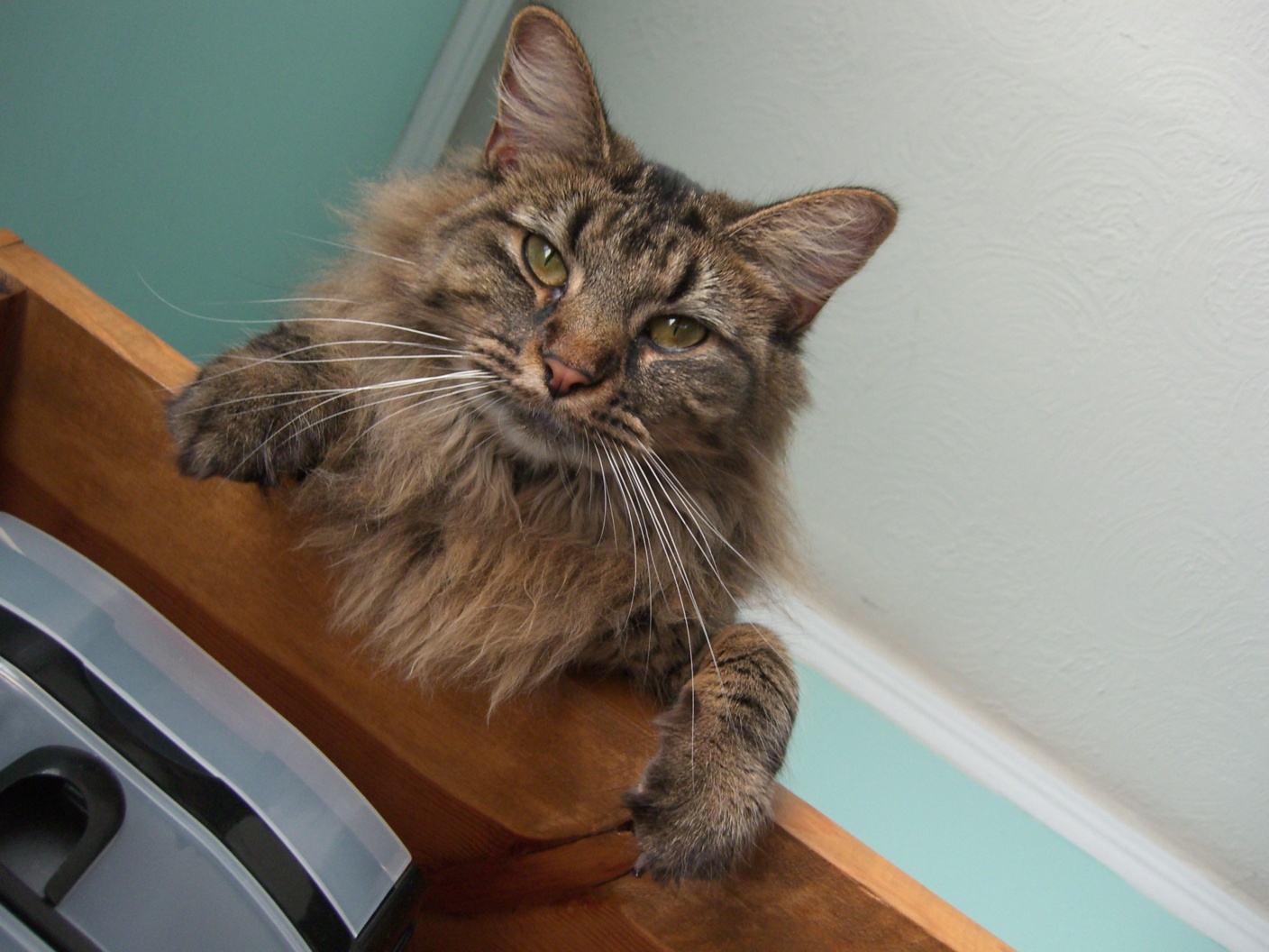
Nutmeg
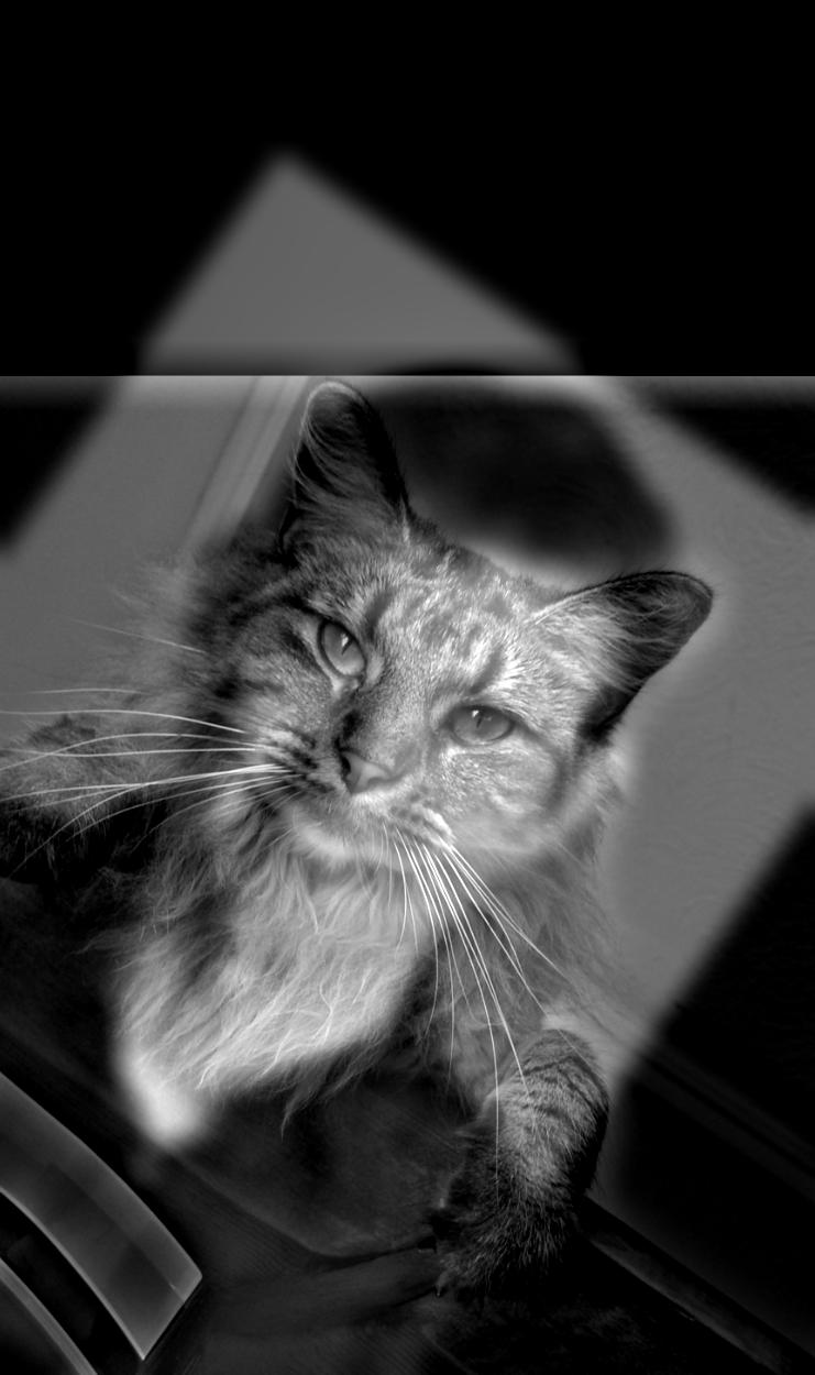
Nutrek
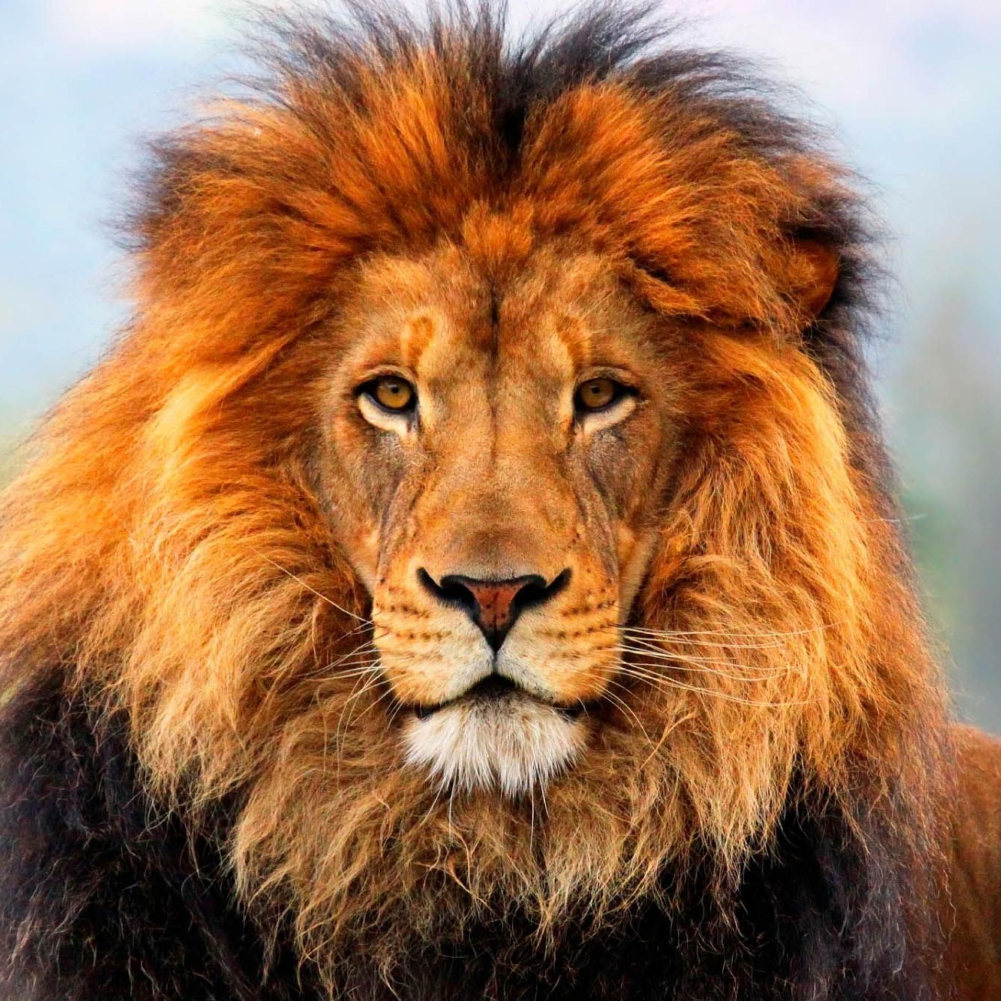
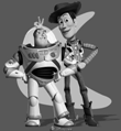
Lion
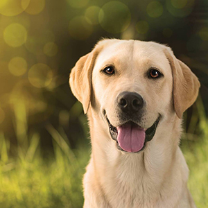
Dog
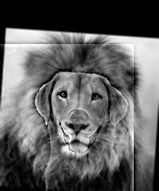
Better Dog
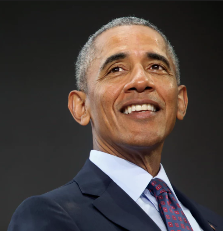
Obama

Trump
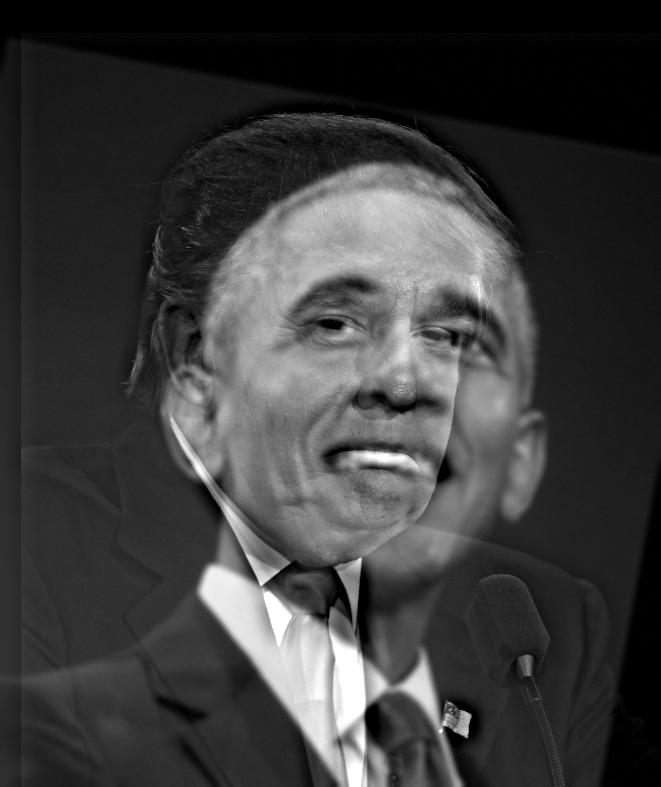
Political Indecision
The Obama + Trump one didn't work out too well because their faces were of different
sizes...
Fourier Analysis
We can also illustrate this process through frequency analysis, by showing the log
magnitude of the Fourier transform of the two input images, the filtered images,
and the hybrid image. We will use the fourier transforms of the Derek and Nutmeg images:
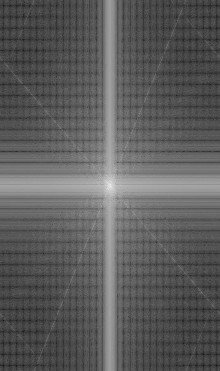
Original Derek
Original Nutmeg
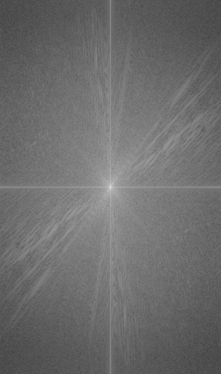
Low Frequency Derek
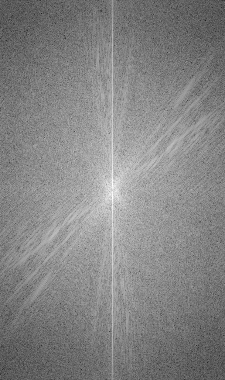
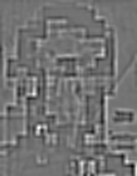
High Frequency Nutmeg
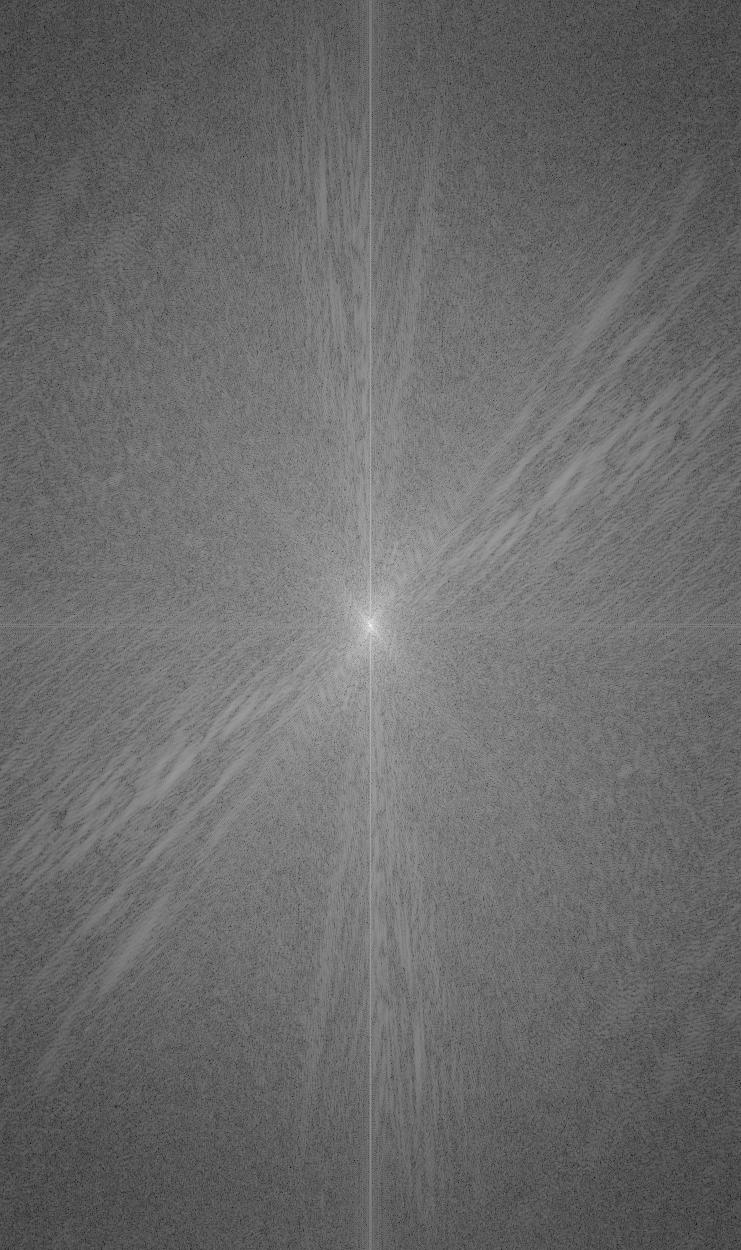
Hybrid Image
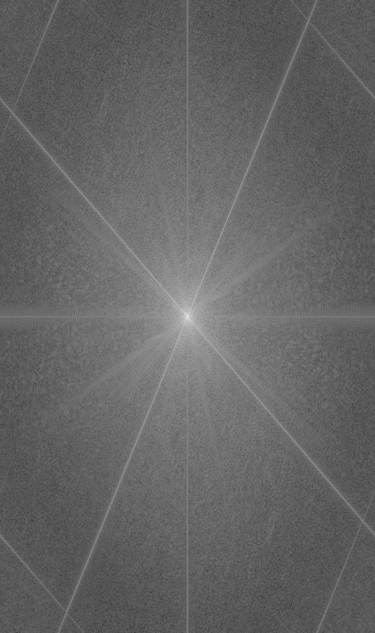
Focusing on the low-frequency/high-frequency/combined transforms, we can see a stark
difference between them. The low-frequency transform is characterized by very distinct
vertical and horizontal lines intersecting at the center. Contrastingly, the high-frequency
transform is characterized by diagonal lines piercing the center, representing the edges in
the image a result of it being rotated when aligned. The transform of the hybrid image thus
makes perfect sense as it is a combination of the transforms of both low-frequency Derek
and high-frequency Nutmeg.
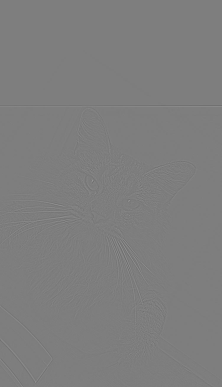
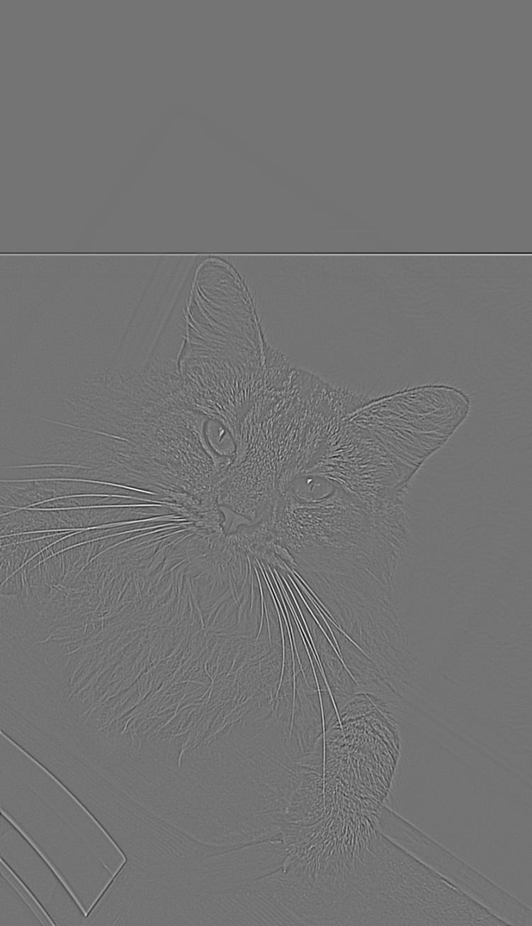
Part 1.3: Gaussian and Laplacian Stacks
We then implemented Gaussian and Laplacian Stacks, very similar to the pyramids we used
in Project 1, but without downsampling. This stacking method involved applying the Gaussian
filter (once again) at each level, exponentially increasing our sigma value of the Gaussian
kernel at each level, but without subsampling. The Laplacian stack was created in a similar
fashion, by adjusting the sigma of the Gaussian kernel at each level, but then getting the
differences between each Gaussian image in the stack.
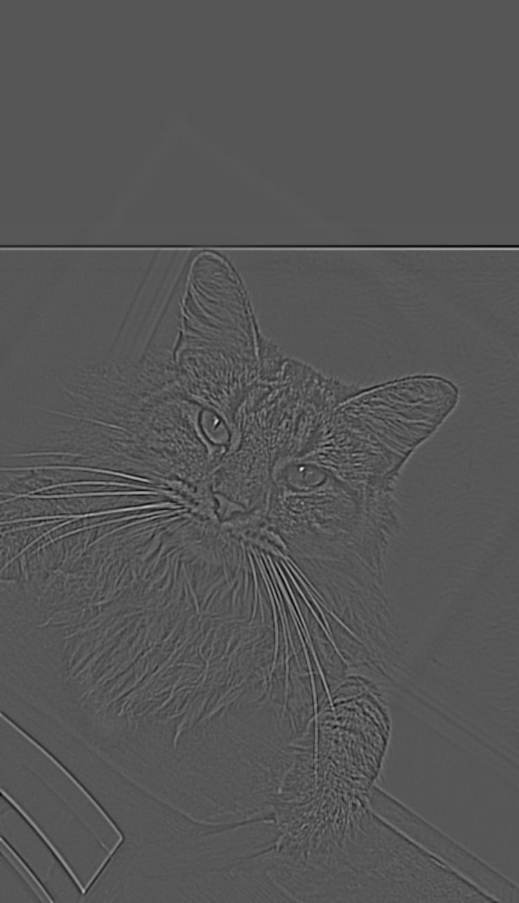
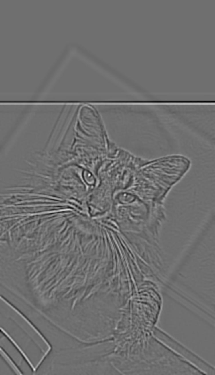
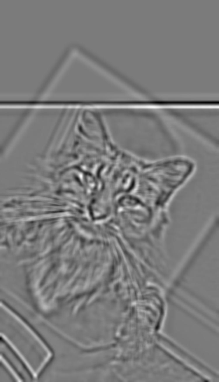
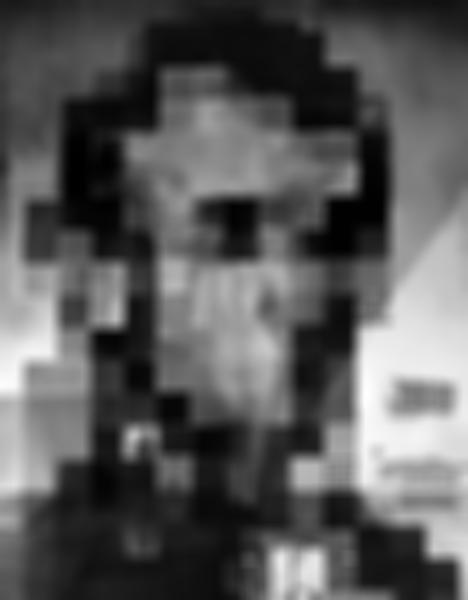
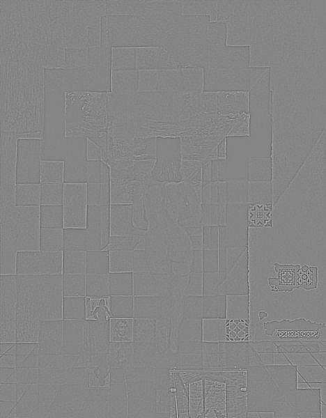
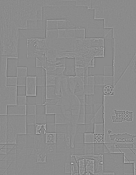
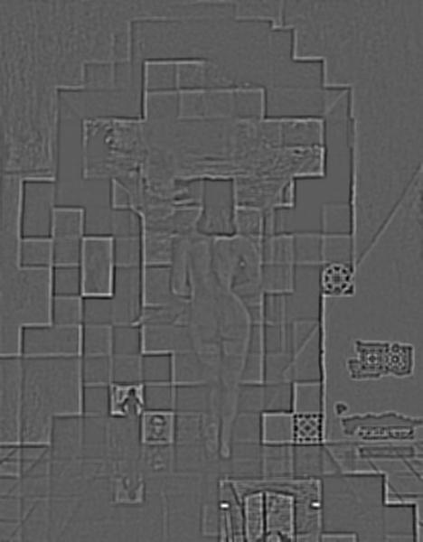
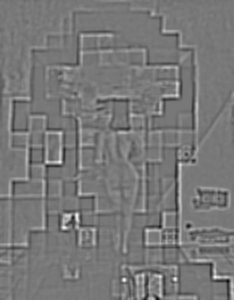
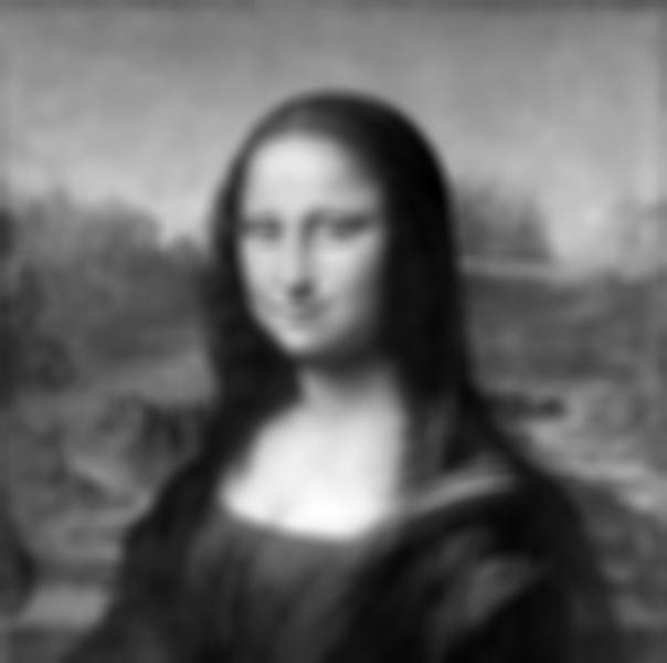
Here are the results of applying this stacking method on our Nutrek hybrid image in part 1.2:
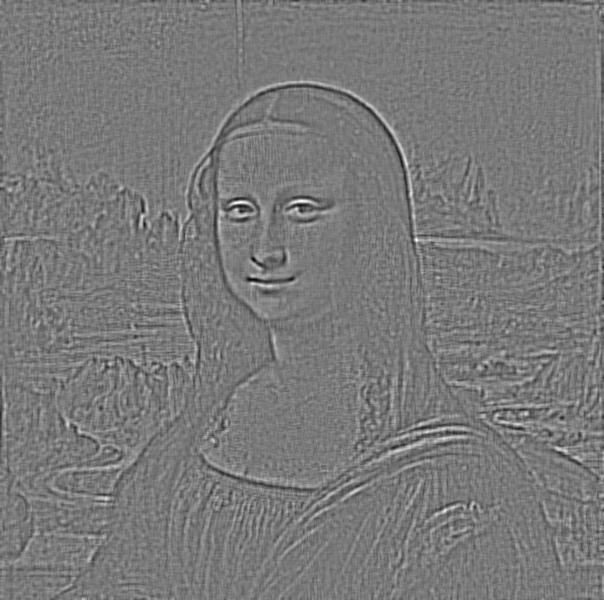
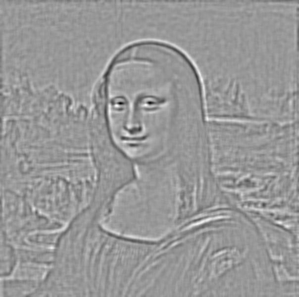
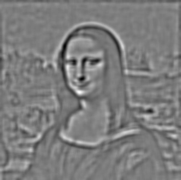
Gaussian Stacks
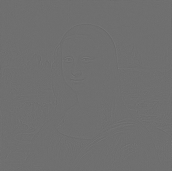
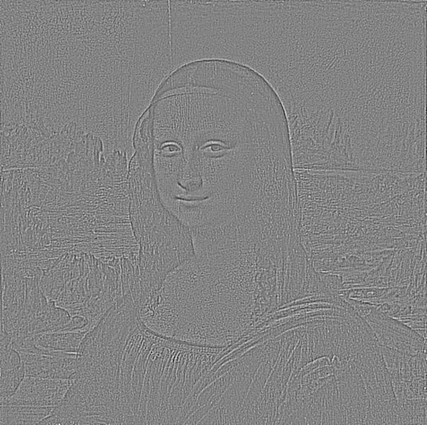
Laplacian Stacks
I also tried creating stacks from images that contain structure in multiple resolutions:
Gaussian Stacks
Laplacian Stacks
Gaussian Stacks
Laplacian Stacks
Part 1.4: Multiresolution Blending
Using what we have learned from previous parts about applying low and high frequency
filters using Gaussian kernels, we move on to Multiresolution Blending, which involves
applying a mask to two images so one occupies one half and the other image occupies the
other, and then computing a gentle seam between the two images at each band
of image frequencies. We do this using the following equation:

In this equation, GA represents the Gaussian stack and LX and LY
represent the Laplacian stacks for image X and image Y.
This is the result from applying this method on images of an apple and orange:

Apple

Mask

Orange
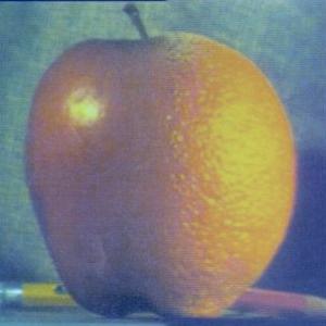
Oraple
Arnold Schwarzenegger + George W. Bush, with another mask:
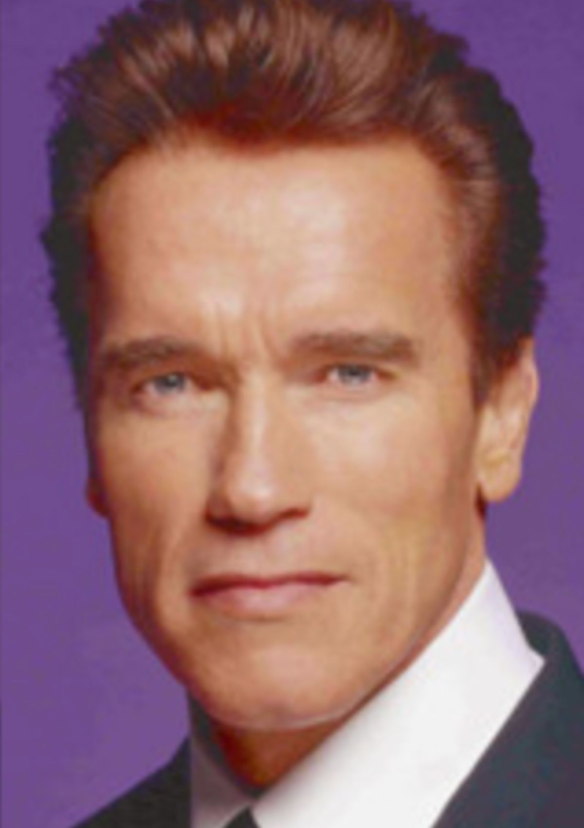
Arnold
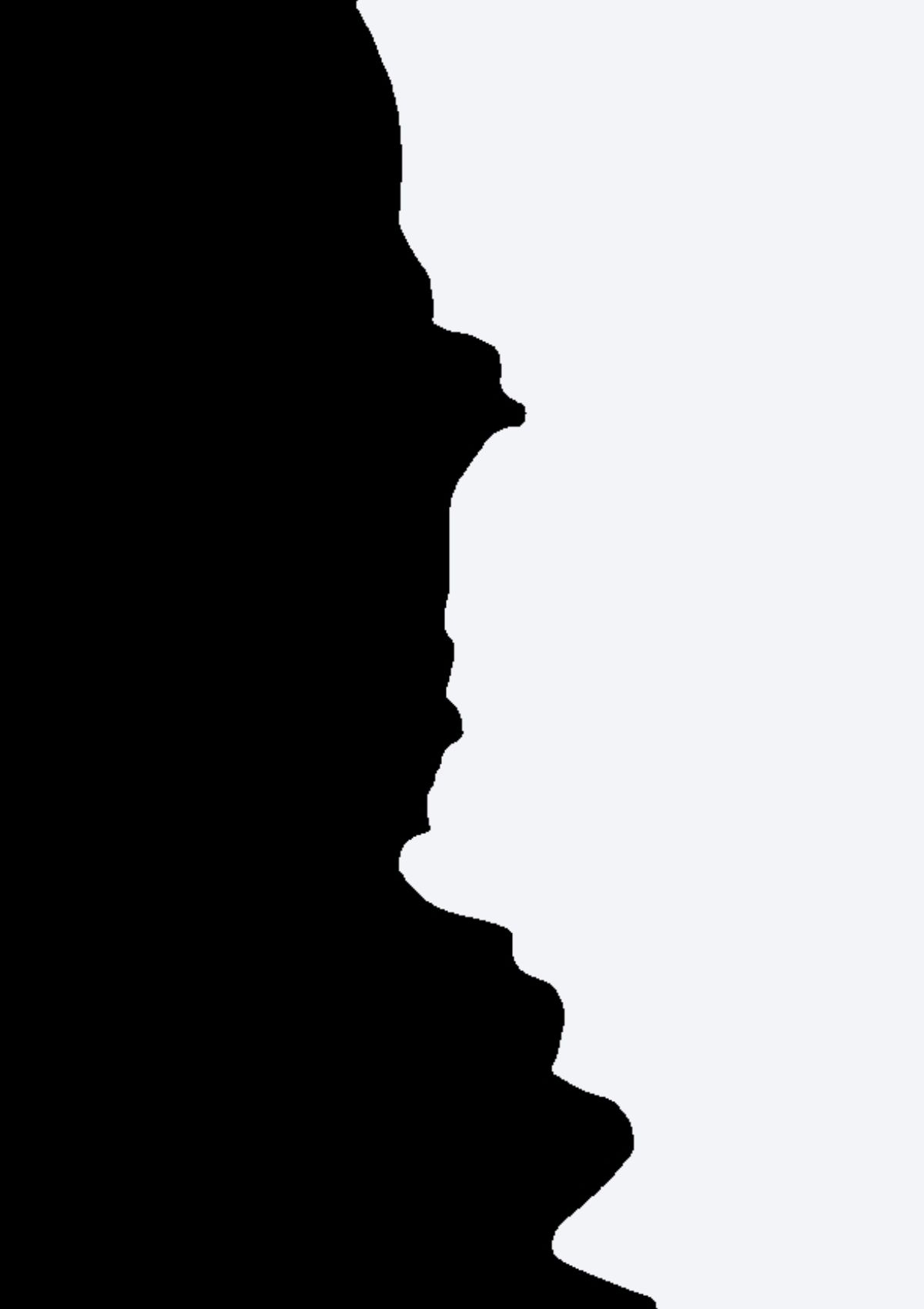
Mask
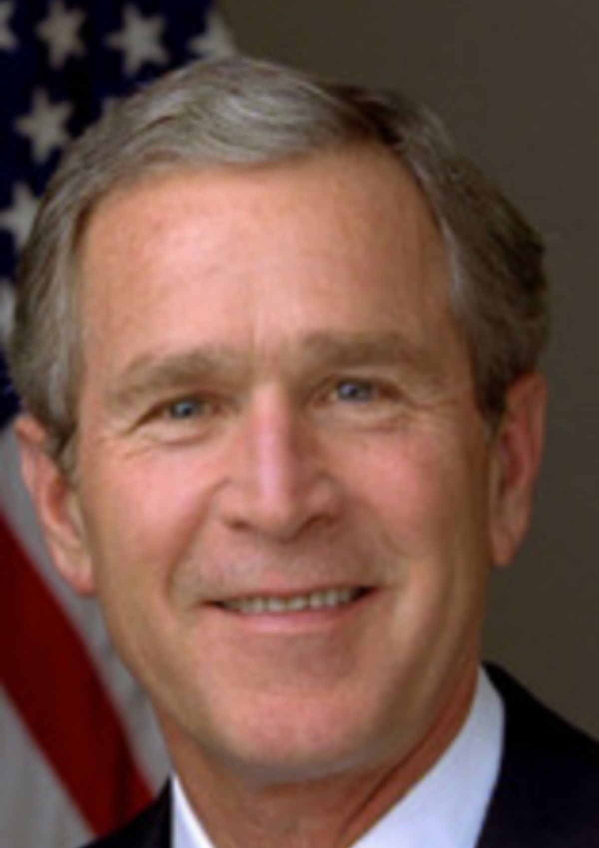
Bush
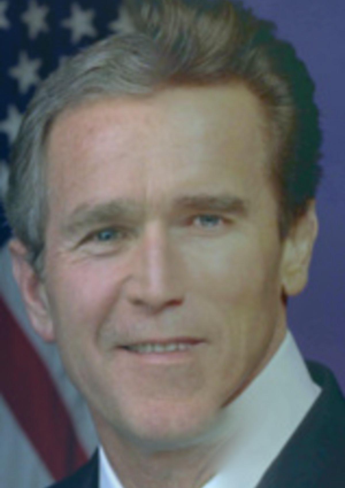
Arbush
Mountains, with and without water, with an even weirder mask:
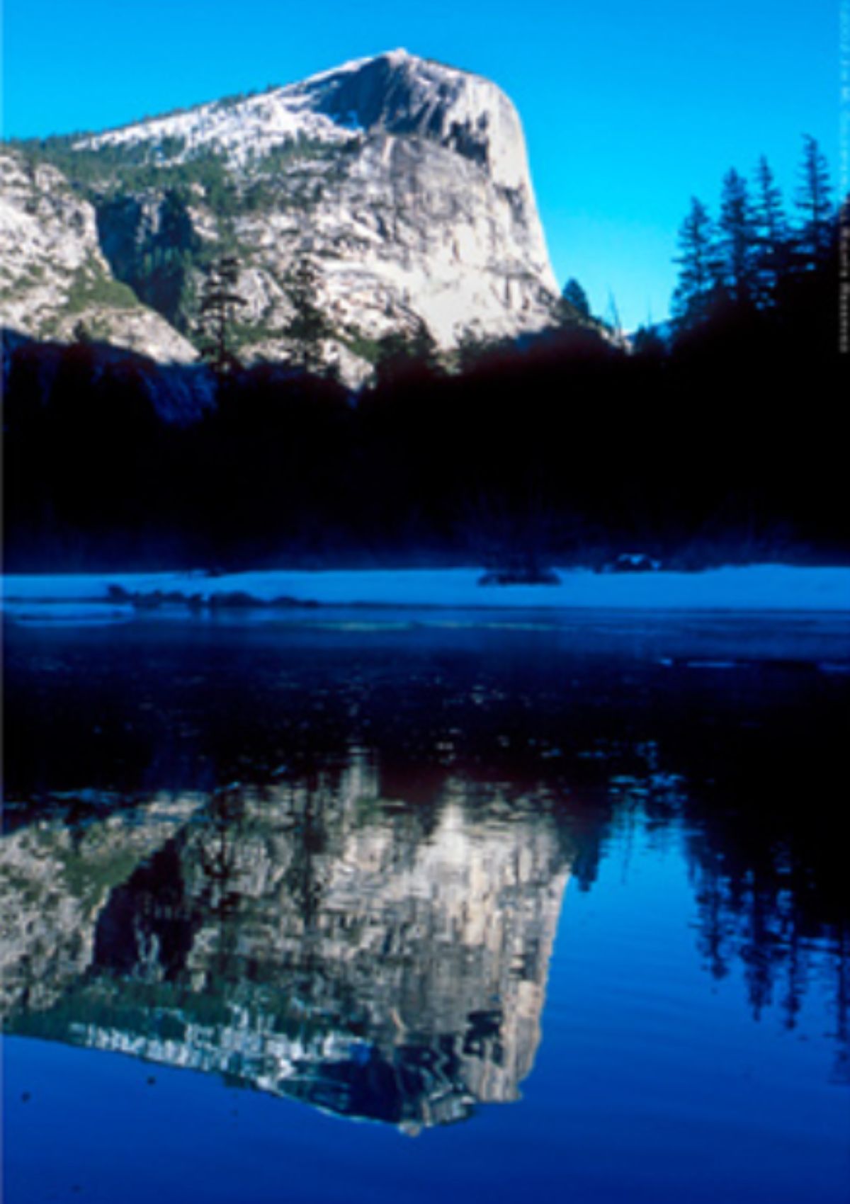
Water
Mask
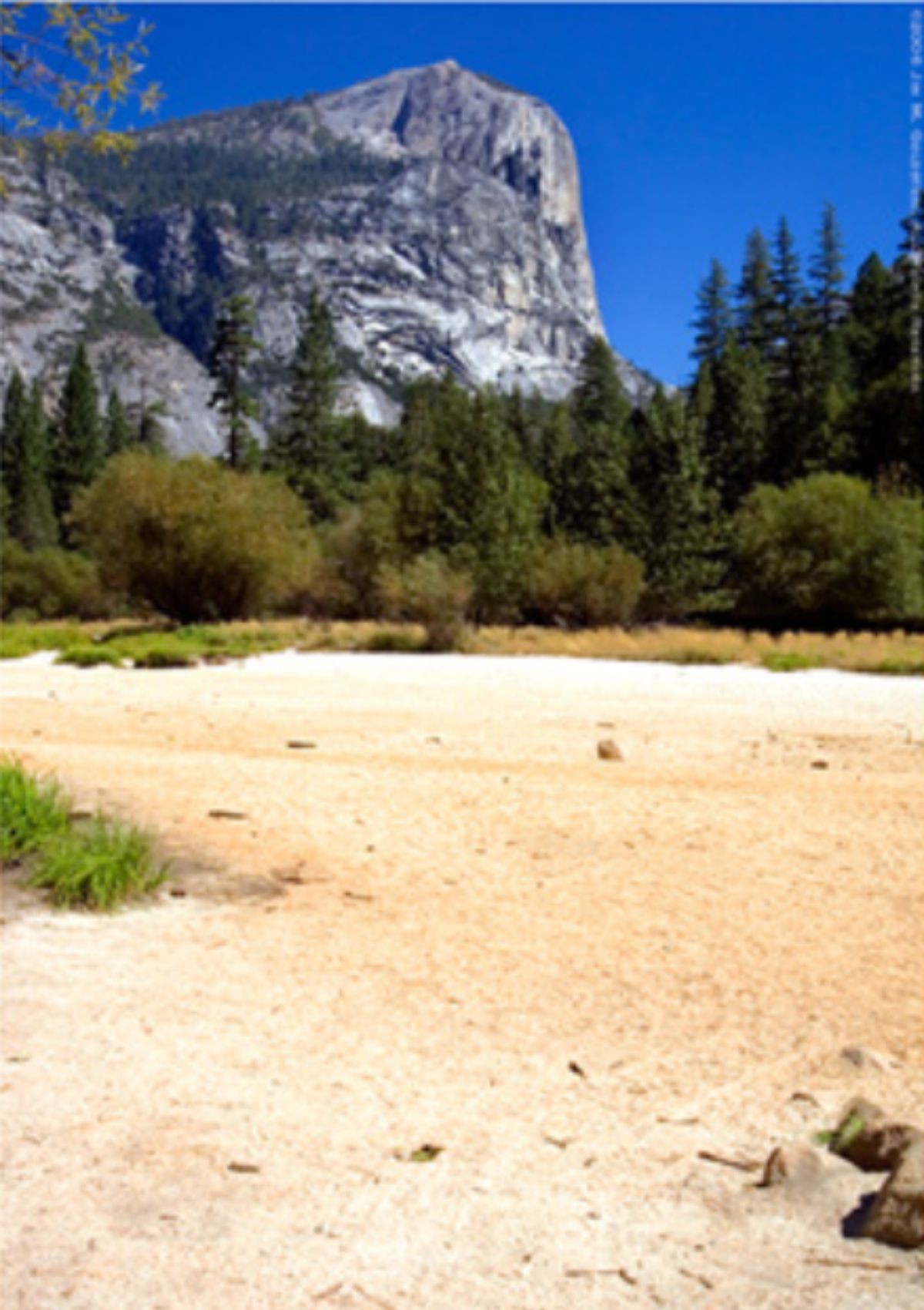
No Water
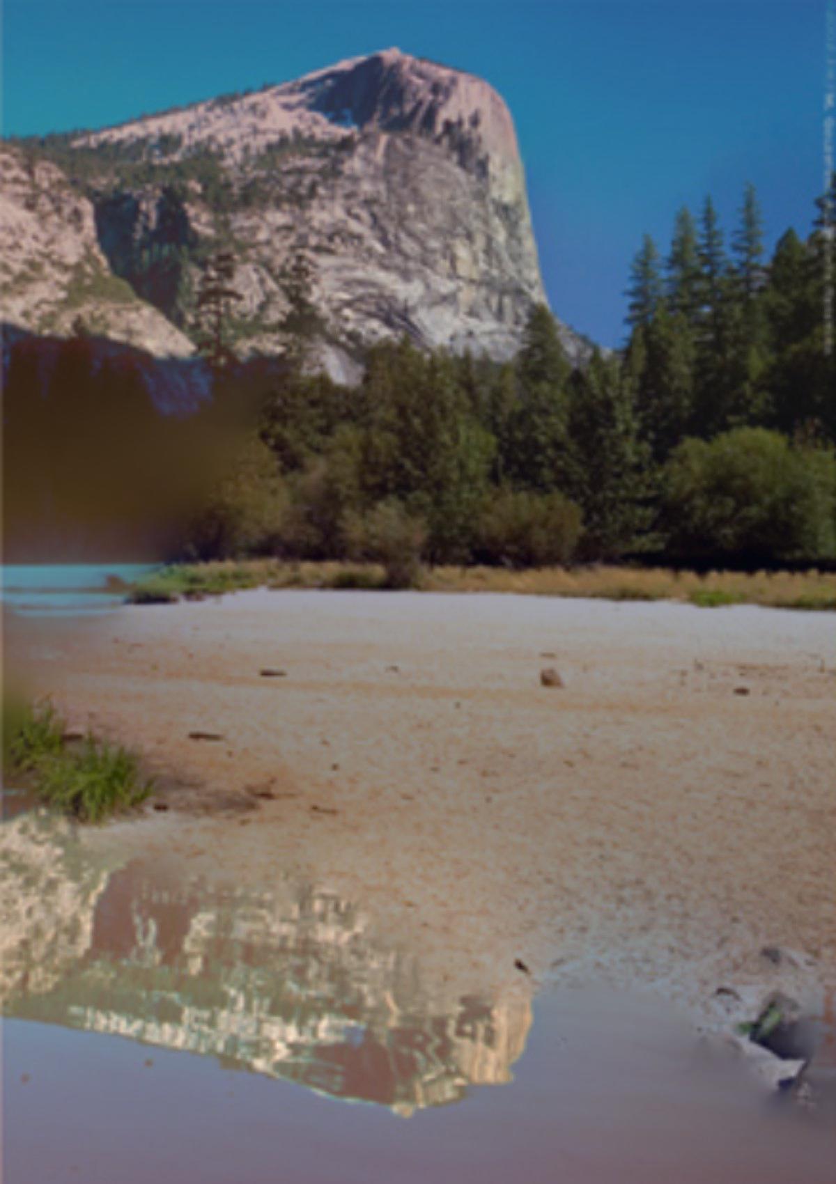
???
Part 2: Gradient Domain Fushion
Project Description
In this part of the problem, we will explore the utilization of gradient domain processing to
blend one image into a cut out section of another image. Gradients simply describe how
the intensity of one pixel differs from another. One can imagine every neighboring pixel
having a gradient from its own neighboring pixels. As humans, we often make use of gradients
to make sense of an image, rather than looking at each pixel intensity individually.
One might ask why we shouldn't just cut and paste an image into another. This is undesirable
simply because of the very obvious seam around the cutout due to the difference in pixel
intensities of the source and target images. Instead of simply cutting and pasting
one image into another, we can preserve the gradients between the original image and the
hole that was cut out. Even though the pixels might be of a different color, the original
form will remain so that the inserted image will look less intrusive and blended in.
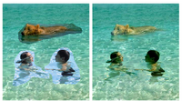
A good example of this blending technique
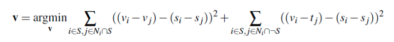
Mathematically, gradient domain processing can be expressed with a least squares
problem, as shown by the equation below:
What this equation essentially describes is that we must minimize the difference
in pixel intensities between the source and target images, thereby guiding the gradient
values of the cutout to match the source image.
Part 2.1: Toy Problem
In this part we are tasked to completely reconstruct an image using the concept
of gradients. Such
a reconstruction can be done by starting with one seed pixel (in this example we
used the top left pixel) and calculating gradients from there to reconstruct every
other pixel in the image.
Original Image

Reconstructed Image using Gradients
Part 2.2: Poisson Blending
Despite the improvement efficiency of the image pyramid method,