Part 1: Frequency Domain
1.1 Unsharp Sharpening


If we have a blurry image that we'd like to 'sharpen', how might we go about doing that? First, consider the opposite of sharpening -- blurring. When we blur an image, for example by applyin a Gaussian filter, we're taking away the details. Then, we can think of sharpening as adding these details back in. We can scale the detail (which is the original image - the filtered image) by some parameter alpha to obtain results as on the left.
1.2 Hybrid Images
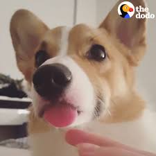
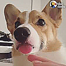
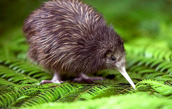
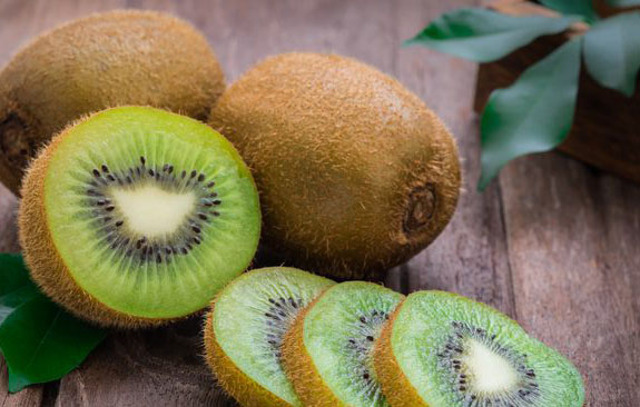
To create these hybrid images, we take advantage of one fact about human perception: our eyes will resolve high frequencies when they are available, but when we are too far away from the image, we cannot detect these high frequencies. Thus, we can create a 'hybrid', where we take the high frequencies of one image and the low frequencies of another, and add them together. I used a simple .5 weight for each half of the image.
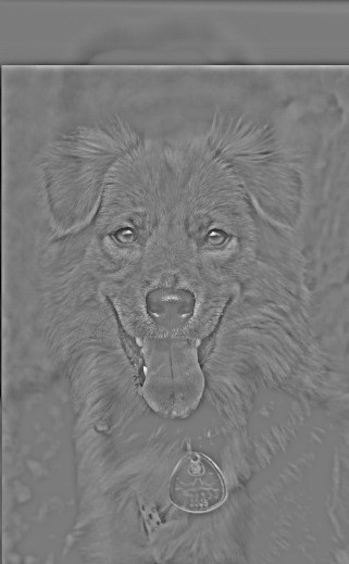
To create the high frequency image, we can subtract the result of Gaussian filtering the image; to create the low frequency image is simply applying the Gaussian filter.
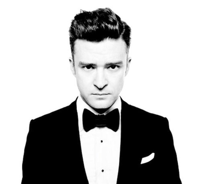
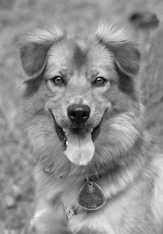
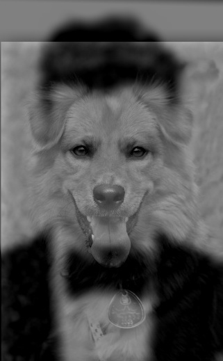
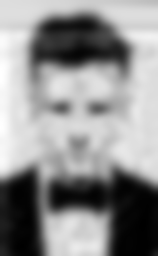
Here, I combined a picture of Justin Timberlake and a good dog.
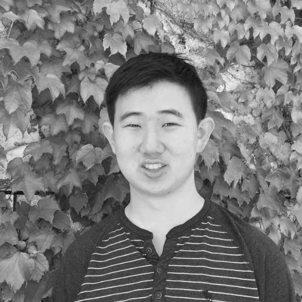
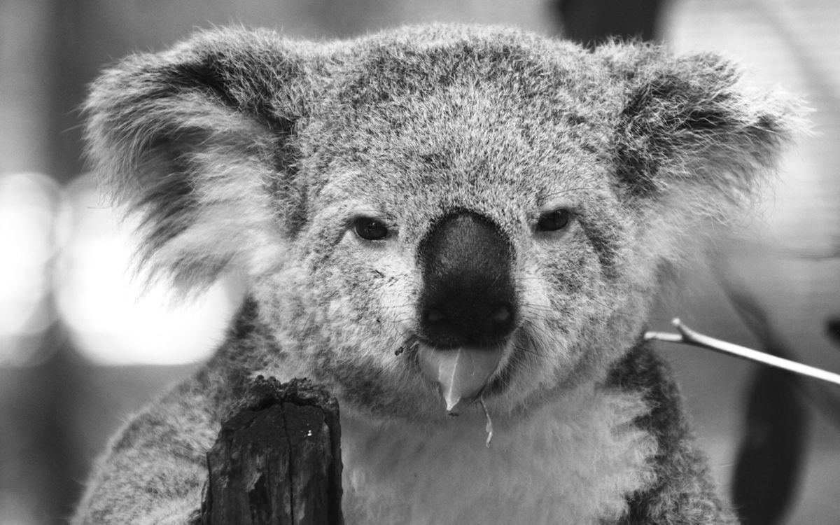
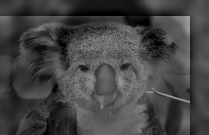
There's a running joke in our friend group that Brandon (also a student in this class) looks like a koala. Here's the proof. (Idea credit: Seiya Ono)
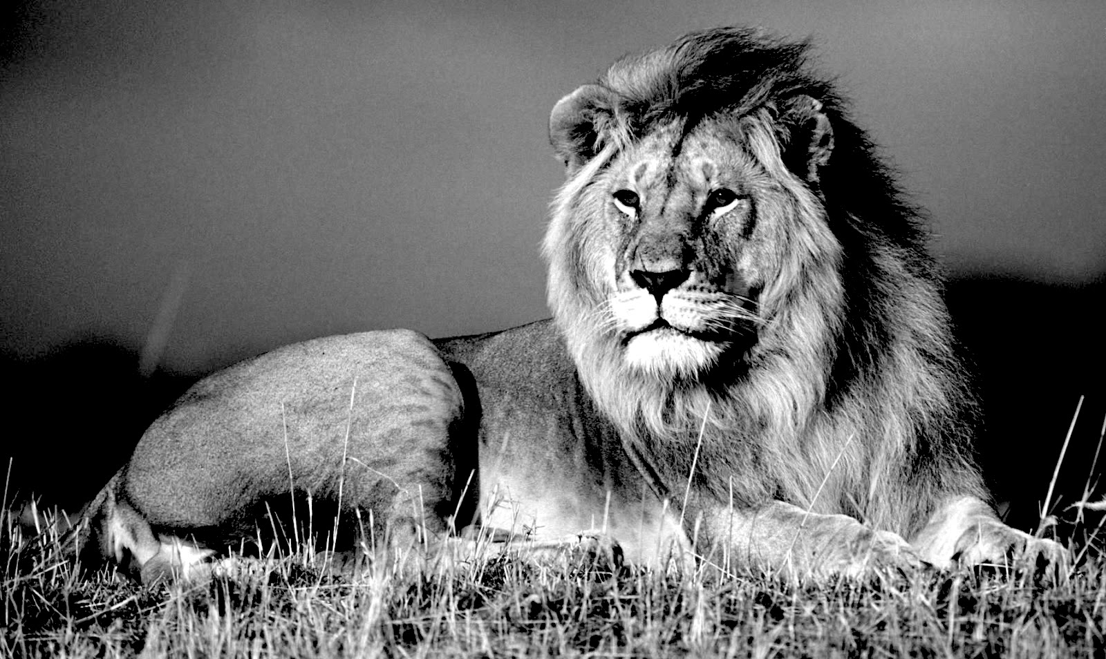
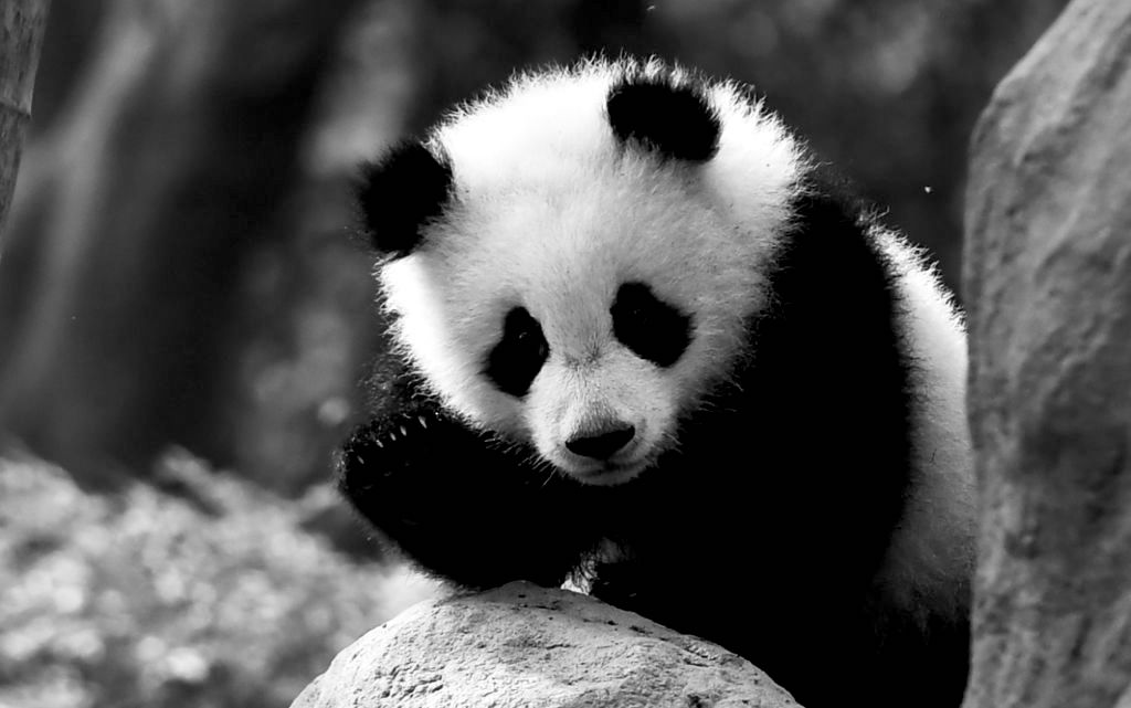
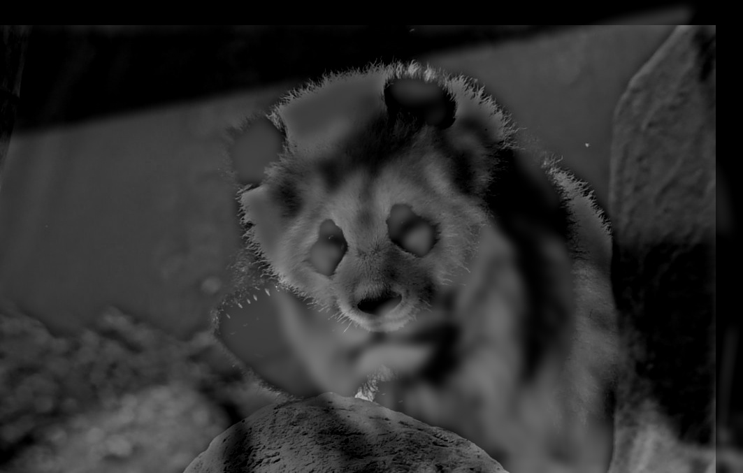
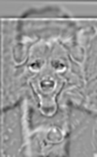
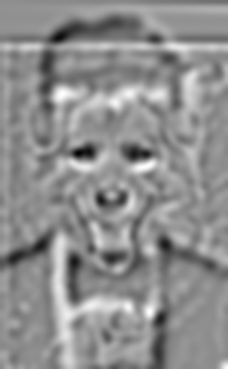
Here's a less successful hybrid image. We attempt to use the panda as the high frequency image, but it is an image with mostly low frequencies. However, its high frequencies are particularly strong. The panda also has very distinct features (ears, eyes, etc.) that don't mix well with the lion. Compare to the Justin Timberlake/dog image, where we use the Justin Timberlake image (with large areas of just black and just white) as the low frequency portion.
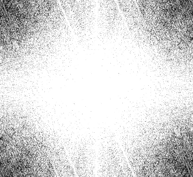
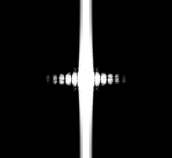
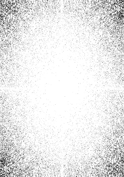
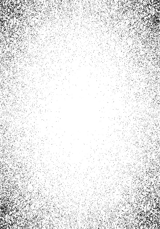
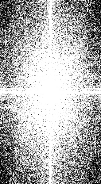
Some frequency analysis images shown below.
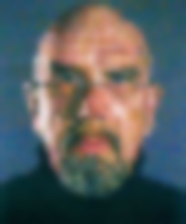
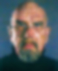
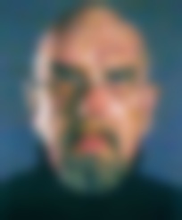
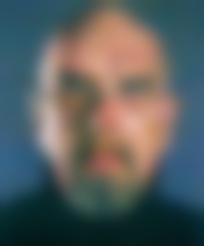
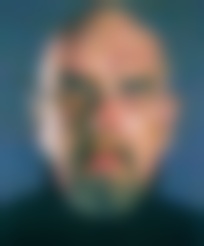
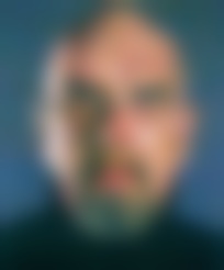
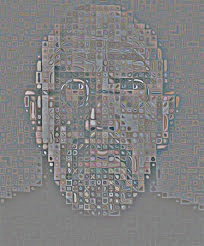
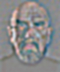
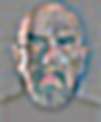
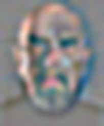
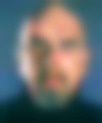
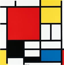
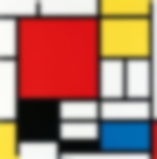
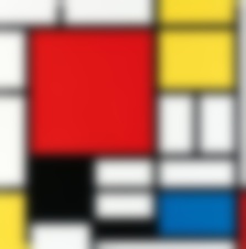
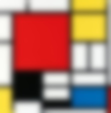
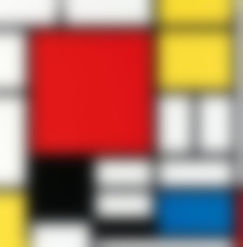
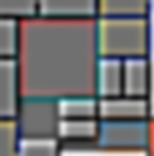
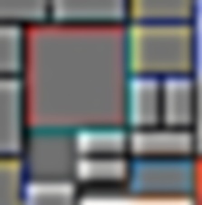
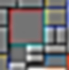
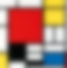
Part 1.3 Gaussian & Laplacian Stacks
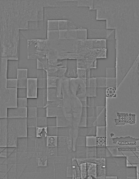
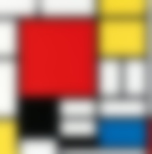
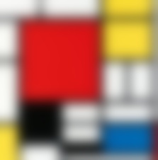
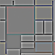
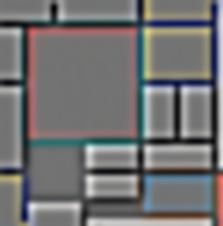
Here, we construct Gaussian stacks by iteratively applying a Gaussian filter (here using width 20) to an image. Below, Level 1 refers to the original image. We also compute Laplacian stacks by calculating the difference between each level of the Gaussian stack (and normalizing for visual clarity). Level 1 of the Laplacian stack is a black image, since Level 1 of the Gaussian stack is the original. Furthermore, the last level of the Laplacian stack is just the corresponding level of the Gaussian stack, so that image reconstruction is possible by collapsing the Laplacian stack.
Source: 'Gala Contemplating the Mediterranean Sea which at Twenty Meters Becomes the Portrait of Abraham Lincoln-Homage to Rothko', Salvador Dali


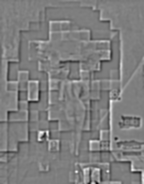
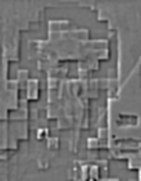
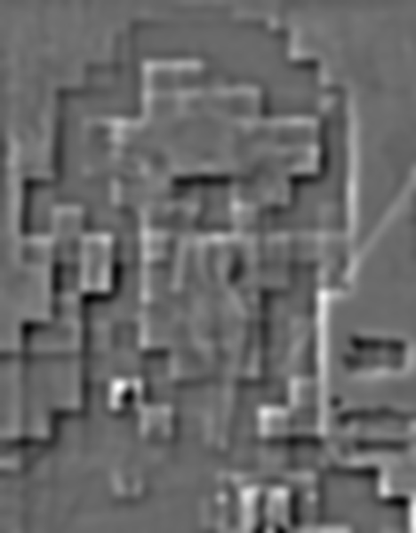


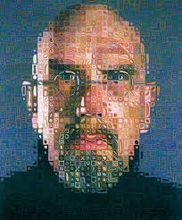
Source: 'Self Portrait', Chuck Close


Source: 'Composition with Large Red Square In...', Piet Mondrian


Source: Justin Timberdog


Part 1.4 Multiresolution Blending
Now that we can create Gaussian and Laplacian stacks, we'd like to combine stacks constructed from different base images, along with a mask, to blend images together with an image spline. This way, we can blend at each band of image frequencies for a much smoother result.
At each level of the Laplacian stacks for each source image, we Gaussian filter the mask to the same level (to also create a smoother spline), then use the mask to do a sort of "alpha" blend between the two source images. Basically, we use the values in the mask to calculate a linear interpolation between the two images.
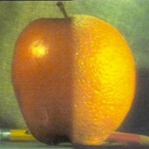
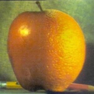
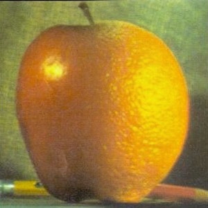
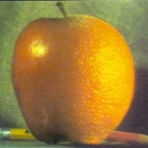
Once I got my 'orapple' working, I wanted to play around to see how changing (1) the width of the Gaussian kernel used, and (2) the number of layers in our stacks, affected the results.
Obviously, increasing both the width of the Gaussian and the number of layers in the Gaussian and Laplacian stacks achieved the best results. However, we can also note that increasing the number of layers while keeping the width low does have a slightly less notable seam than increasing the width while maintaining the number of layers.
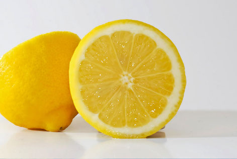
Now that I got this little experiment out of the way, I went ahead and created a couple other blended images with the 'maximum' width and layer depth shown here. Sticking with the fruit theme:
Part 2: Gradient Domain Fusion
Part 2.1 A Toy Problem
To warm up a bit, we begin with a toy problem - reconstructing a single image by its gradients. Given the following image (or indeed, any image), we can construct a `b` vector that consists of all the x and y gradients from an image, as well as a single pixel's intensity. Then, we can construct a corresponding `A` matrix, such that using least-squares to solve the equation Ax=b will yield the original image in the `x` vector.
Here, I set `i` to be the current pixels and calculated the gradients of i and the pixel to its right, and below it. I handled edge cases by simply setting to the value of the pixel on the boundary -- no gradient calculated.
I construct `b` in linear time with respect to the number of pixels in the image, then use a sparse matrix creator and linear squares solver to obtain the original image back.

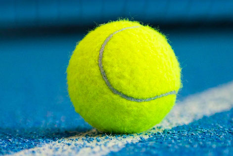
Part 2.2 Poisson Blending
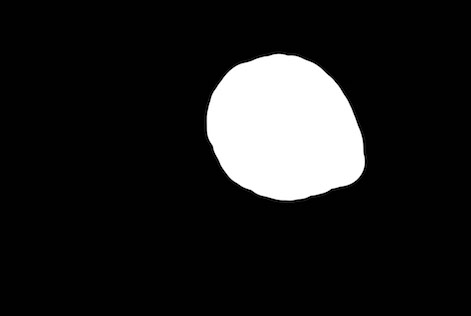
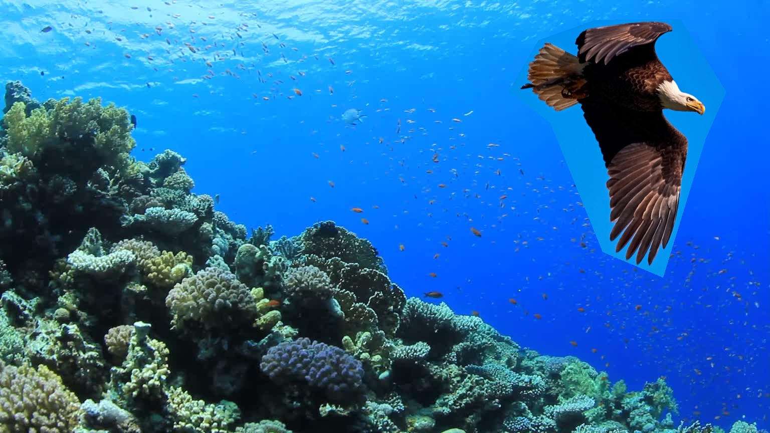
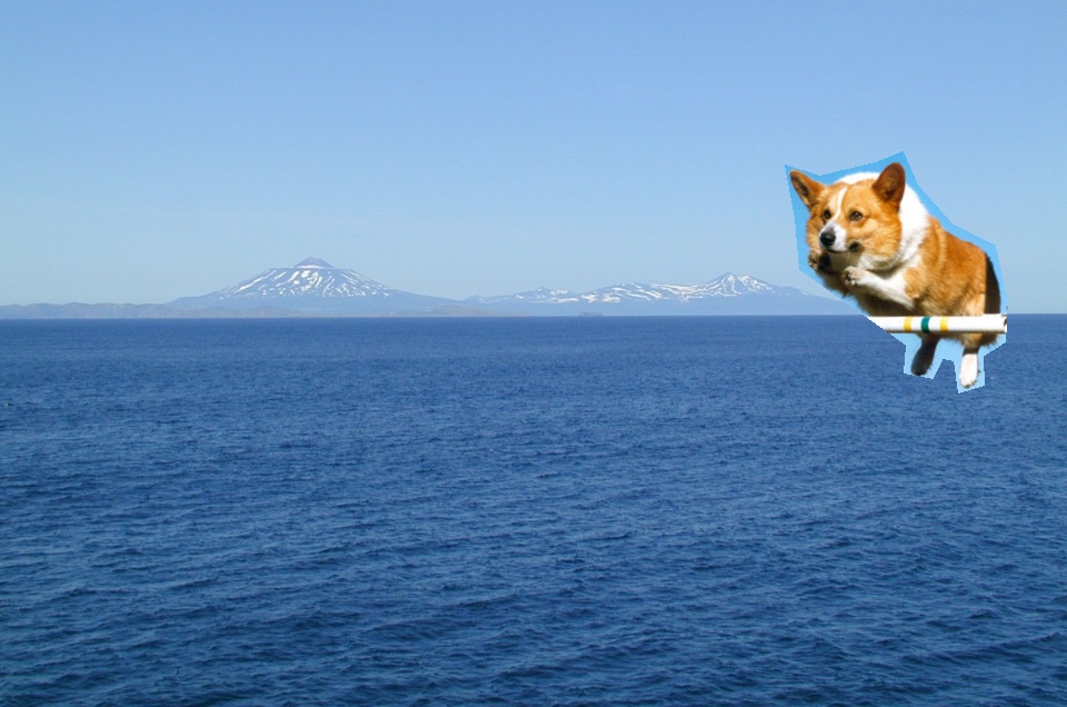
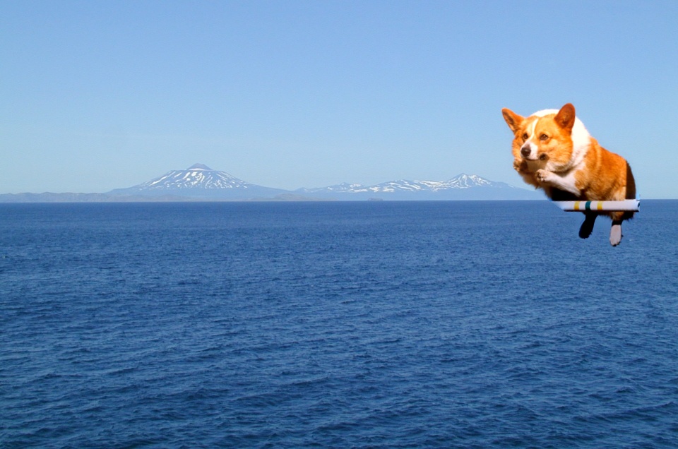
Now we can move on to the exciting stuff! With Poisson Blending, we can "copy" part of one image into another, but using our friendly gradient domain in order to create a smooth transition between the source and the target.
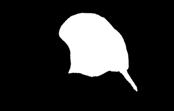
For every composite image we'd like to create, my method requires 4 or 5 pieces: (1) the target image, where you'd like the source to be pasted in, (2) the source image to cut out from, (3) a mask for the target image, where the white parts of the mask correspond to where the source will be pasted in, (4) a mask for the source image, where the white parts are the parts of the source we'd like to transfer, and optionally (5) a transformed version of the source image -- needed if you rotated or resized the source image. A big thank you to fellow student Nikhil Uday Shinde for sharing his mask creating code!!!
My method was to follow the following:
For each pixel in the masked region,
- Get each pixel in its 4-neighborhood: the pixel to the left, to the right, above, and bliow it.
- Calcliate the gradient between the 'center' pixel and each of its neighbors.
- If the neighbor is outside the masked area, also add in the corresponding pixel value from the target image.
- Store each of these gradients in `b`.
- Simlitaneously calcliate the corresponding row, column, and data information to generate the sparse `A` matrix after all this.
Thus, this runs linearly in the number of pixels in the mask (which can still be quite long). This portion takes up the majority of my runtime, as the creation of `A` and least squares solving does not take too long. Note that most gradients within the mask are actually "double counted", since I include each of the four neighbors for every pixel in the mask. However, this makes it much more convenient to program. Additionally, I experimented with just setting the gradient where one pixel was outside the mask to just the corresponding target pixel, but did not notice any difference. The results shown use the method described in the list above.
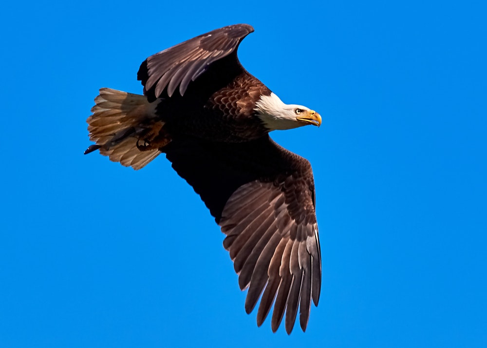
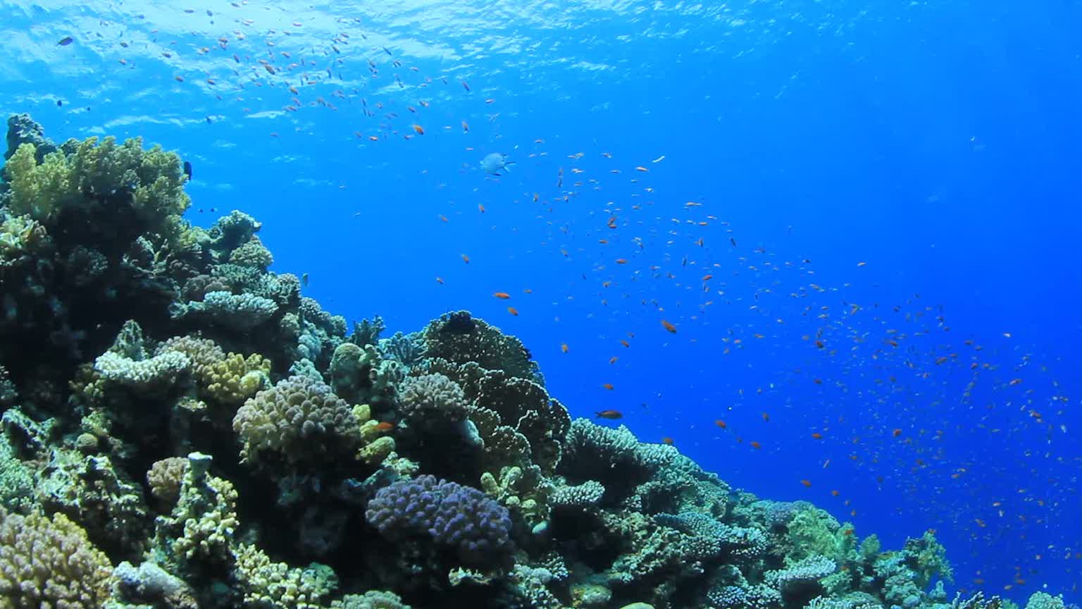
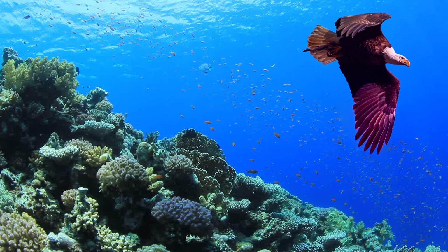
Eagle in the Water
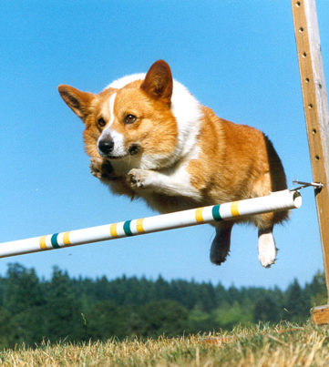
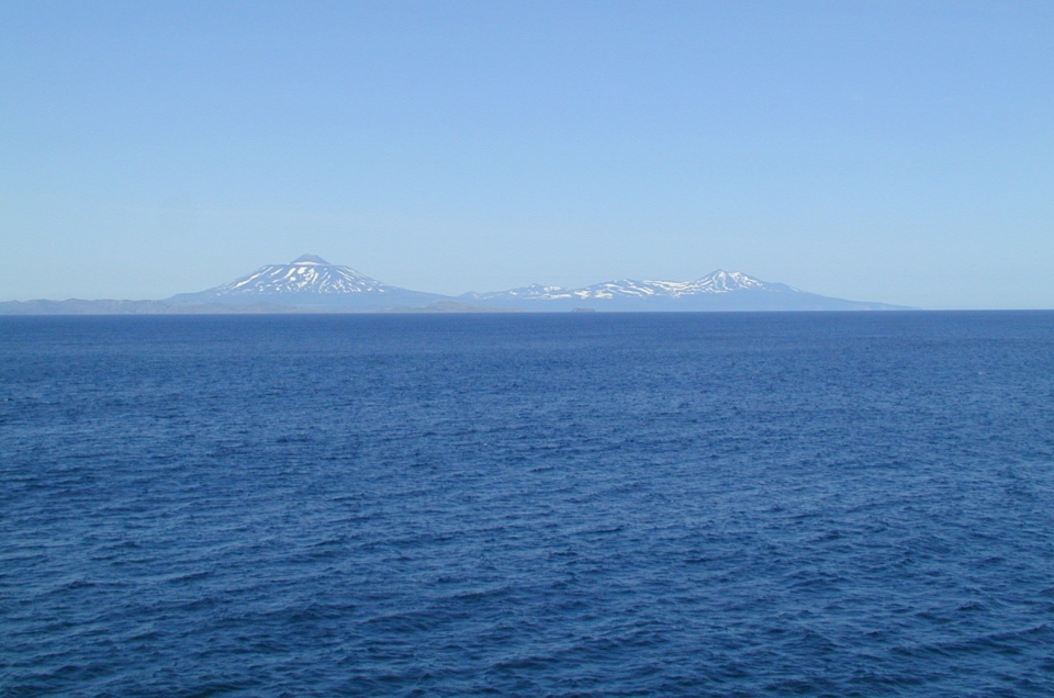
Corgi at Sea
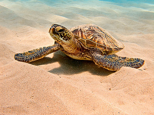
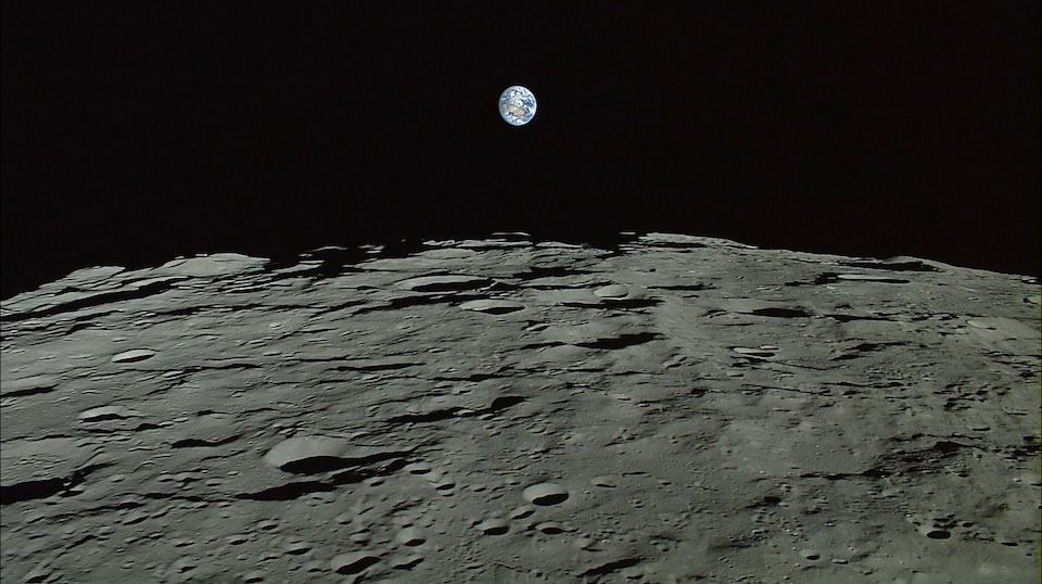
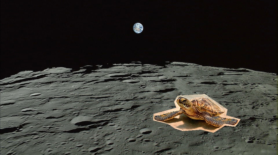
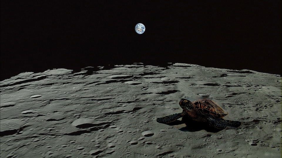
Turtle on the Moon
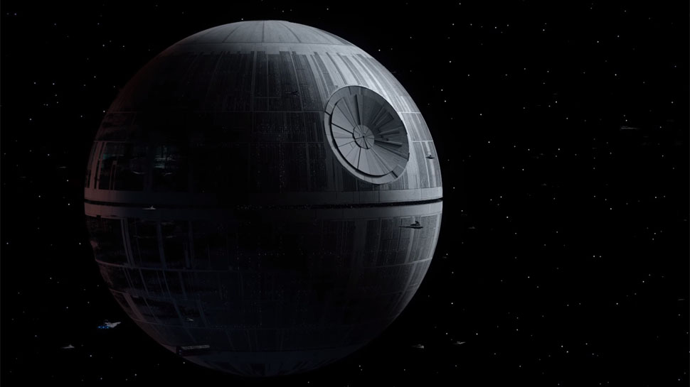
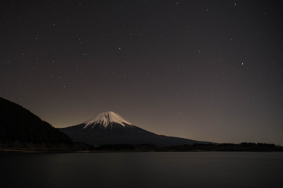
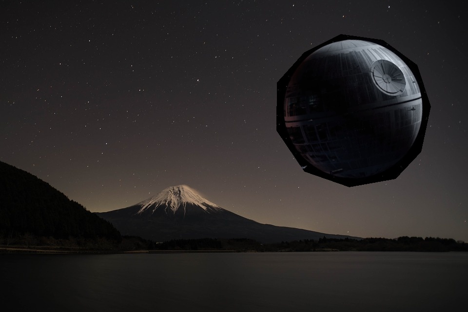
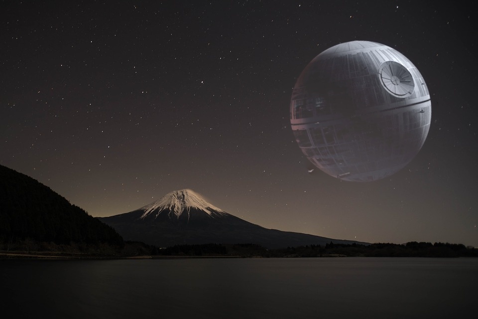
Death Star Over Japan (!! My personal favorite)
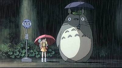
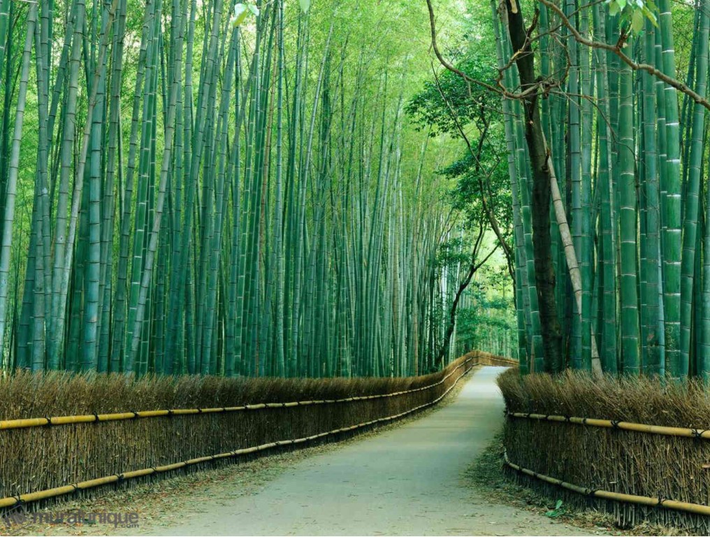
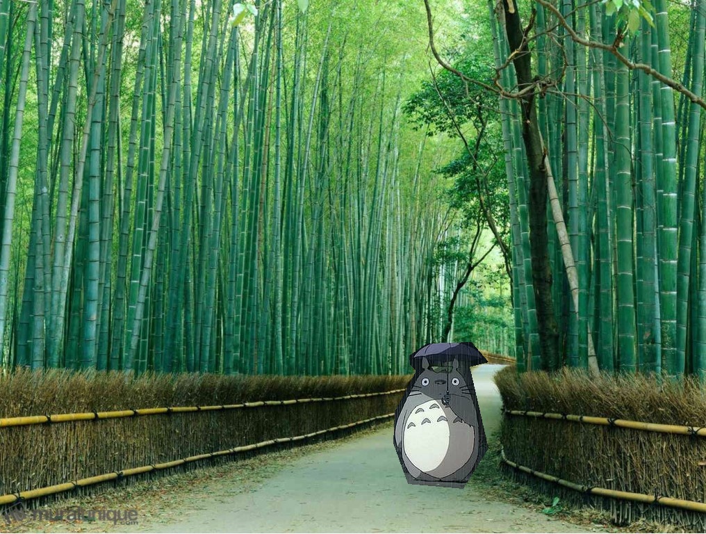
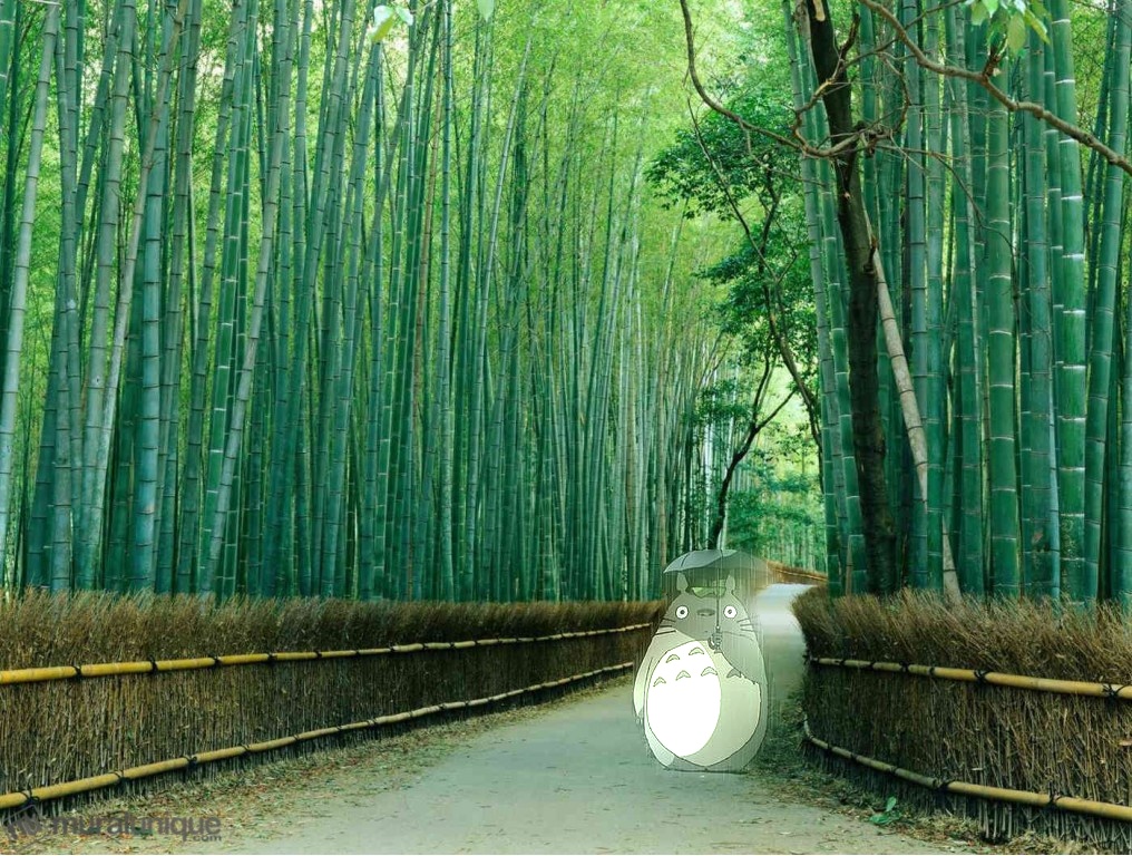
Totoro in Real Life
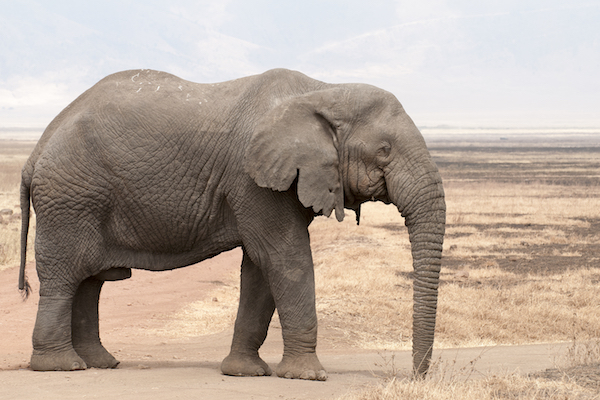
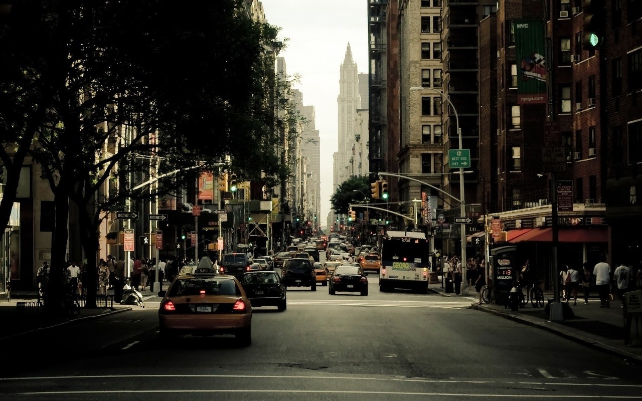
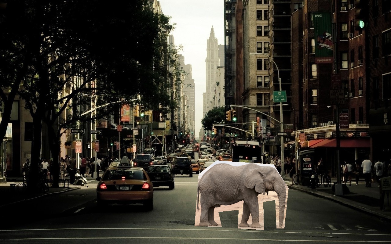
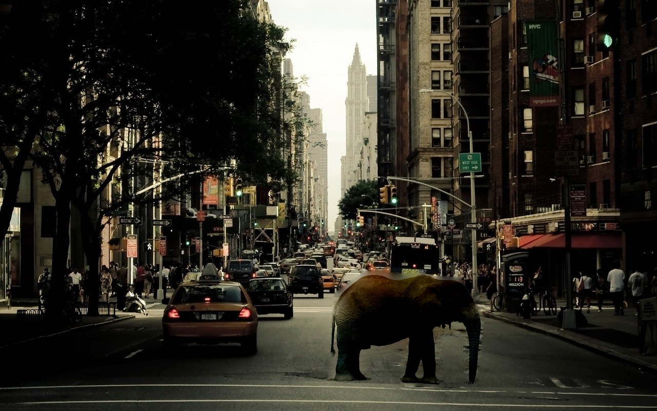
Less Successful: Elephant in the City
Less Successful: Dogs & Dolphins
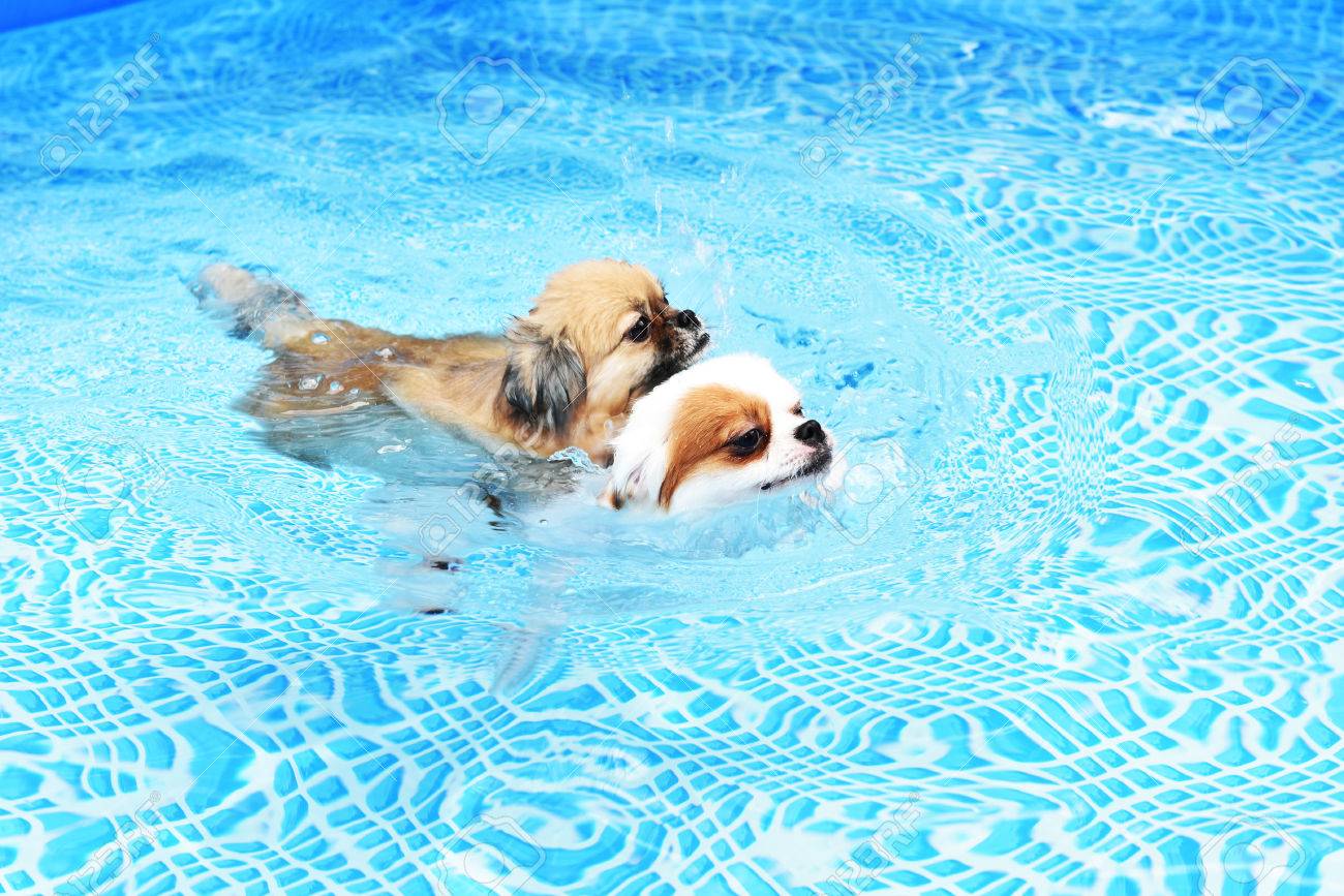
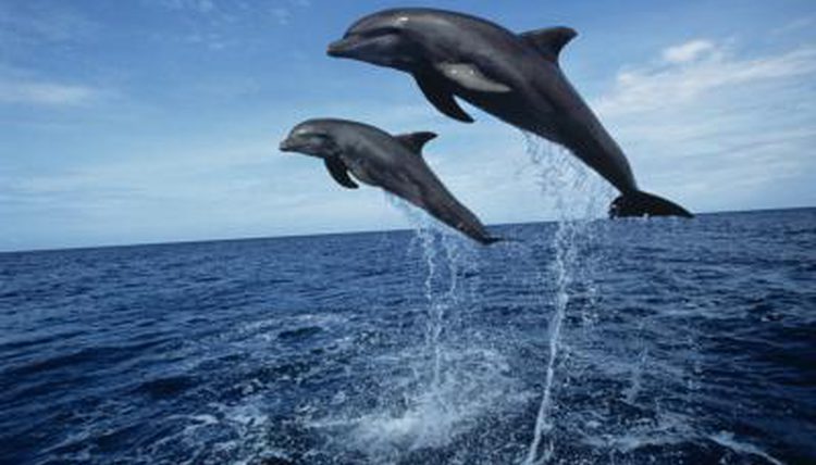
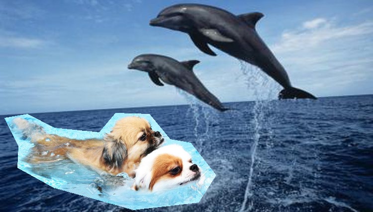
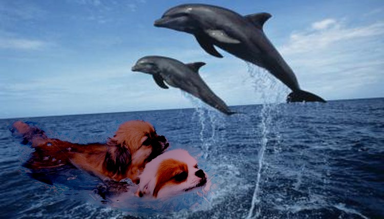
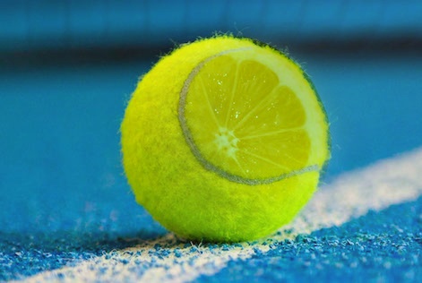
In these last two cases, we notice failures for two main reasons -- the gradients in the source image are fairly complicated, and they also differ quite greatly from the target region. Thus, we can see a fairly clear border around the masked region. For comparison, we can look at the Turtle on the Moon and Totoro in Real Life composites. Both of these are fairly different compared to the target region, and result in highly modified values inside the masked area. However, we can still resolve the border fairly well in those cases.