Project 3: Fun with frequencies and Gradients
Louise Feng
Part 1.1: Warmup
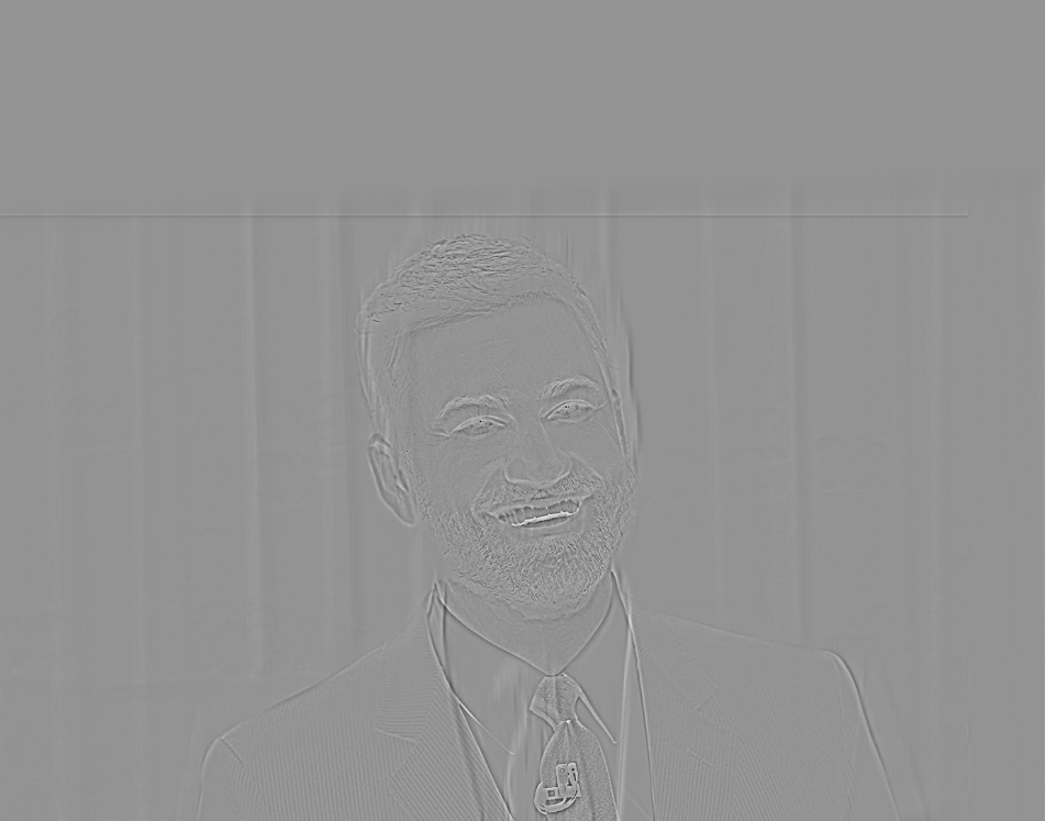
To sharpen an image, I used the unsharp masking technique. Given an input
image and a Gaussian kernel as a filter, we apply the convolution to sharpen
the image. I used the OpenCV library for Python to create a 9x9 Gaussian kernel
with sigma = 10. I then filtered the image by the kernel to create the unsharpened
image, and computed :
Original + alpha * (original - unsharpened)
Where the alpha chosen was 0.5. The result is an image with heightened edges
and therefore seem sharper.
Part 1.2: Hybrid Images
In this part, we take 2 images and blend them together to create one hybrid
image. The end result is an image where one of the original images is more
apparent from a distance and the other from up close. This is achieved by
taking the high frequencies of one of the images and the low frequencies of
the other. The process to create the filters is very similar to the previous
part. The lowpass filter is the result of filtering with a Gaussian kernel
and the highpass from subtracting the Gaussian-kernel filtered image from
the original. Adding the 2 together (after they've been aligned) creates the
hybrid image.
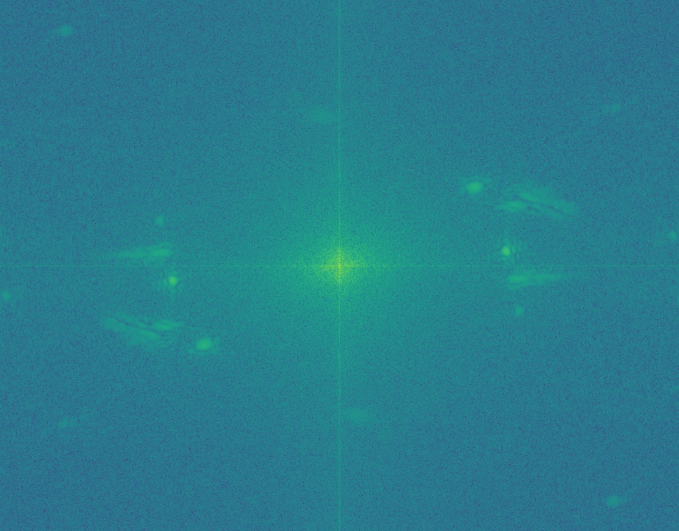
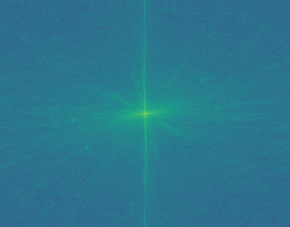
Results and Requency Analysis
Failure Image:
Not every hybrid turns out perfected. In order to look good, the 2 images
should share a few general common features to blend together. Some things
just aren’t meant to be put together. Case in point:
Part 1.3 Gaussian and Laplacian Stacks
Next, we create Gaussian and Laplacian stacks. When applied to images that
contain structure in multiple resolutions, these stacks reveal the structure
at each level. Gaussian stacks are created by filtering repeatedly with a
Gaussian kernel while Laplacian stacks take the difference between the
current land last level of the Gaussian stack. In the following images, the
top row is the Gaussian stack and the bottom is the Laplacian.
Part 1.4: Multiresolution Blending
We use multiresolution blending in this section to create a smooth seam between
2 images and effectively blend them together. To do this, a Gaussian stack is
created from a mask of ones and zeros that denotes where the seam will go. A
Laplacian stack is created from the 2 images. At each layer, we combine the
three and the final result is the sum at each layer.
Part 2: Gradient domain Fusion
In the previous part of the project, we blend 2 images together using Gaussian
and Laplacian stacks. We now blend 2 images together using Poisson blending.
The idea here is to preserve the gradients in the source image (the image
that is blended into a target image) without changing the target image.
However, the pixel intensities after processing the source image will change.
We do this through a least squares problem that creates the pixels inside the
source area of the final image such that:
- For each pixel and its neighbor where both the pixel and its neighbor are
inside the source region, we guide the gradient between them to match the
gradient in the source image.
- For pixels at the boundary where a neighbor is in the target image region,
we look at its neighboring pixel in the target and do the same.
Note that we look at four neighbors (up, down, left, right) to get 2 gradients
(x, y).
Explicitly, the least squares problem we solve is: