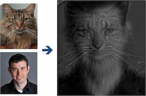
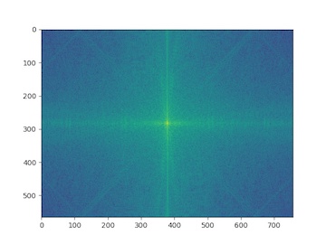
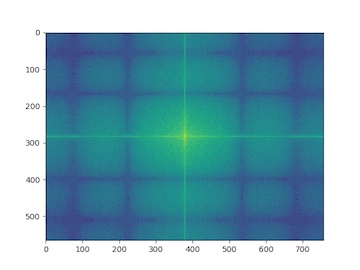
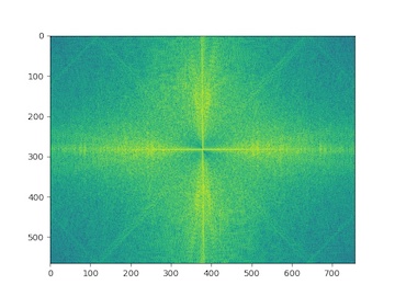
Part 1.3 Gaussian and Laplacian Stacks:
All images are processed with 45x45 Gaussian filter, with sigmas = [2, 4, 8, 16, 32]
The Laplacian image is grey-balanced to demonstrate its structure
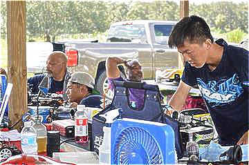
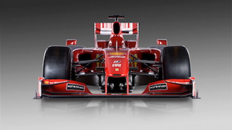
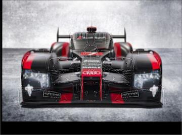
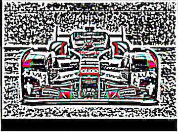
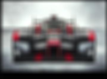
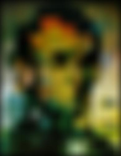
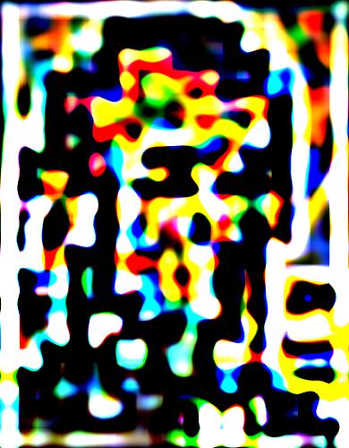
Original image: f1-lemans blend
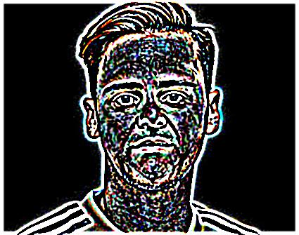
Original image
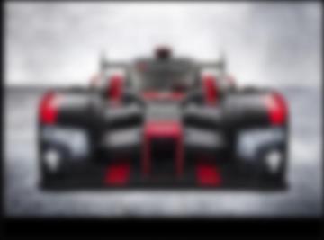
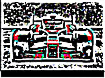
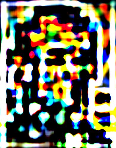
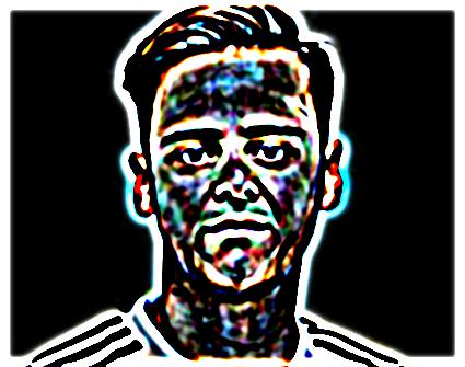
Gaussian stack: sigma = 2

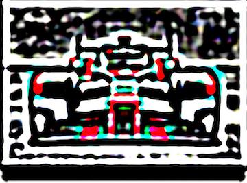
Gaussian stack: sigma = 4

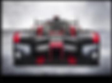
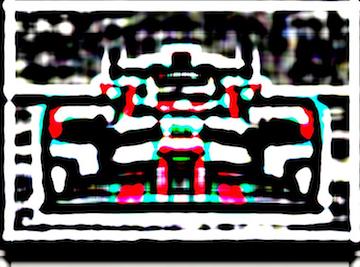
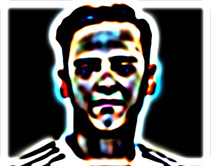
Gaussian stack: sigma = 8
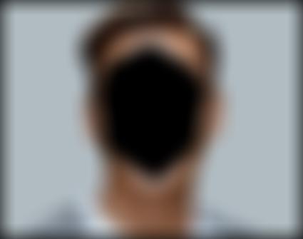
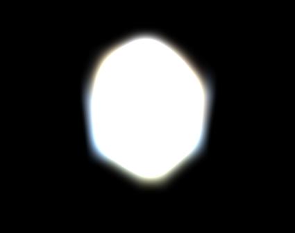
Gaussian stack: sigma = 16
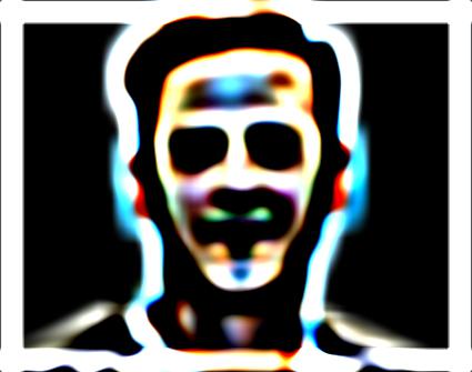
Gaussian stack: sigma = 32
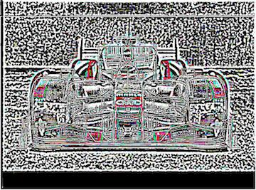
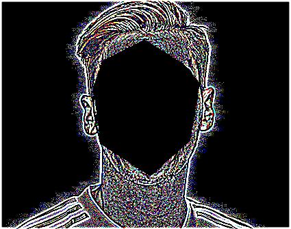
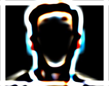
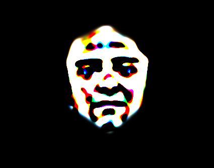
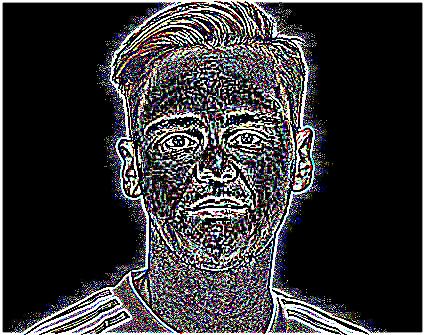
Laplacian stack: 1-2
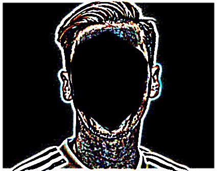
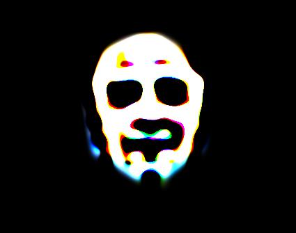
Laplacian stack: 2-4
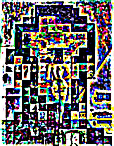
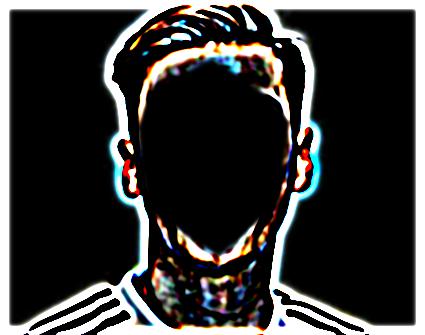
Laplacian stack: 4-8
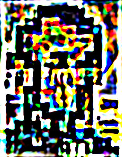
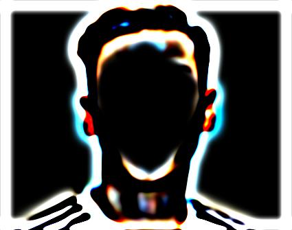
Laplacian stack: 8-16
Laplacian stack: 16-32
Laplacian stack: Remains
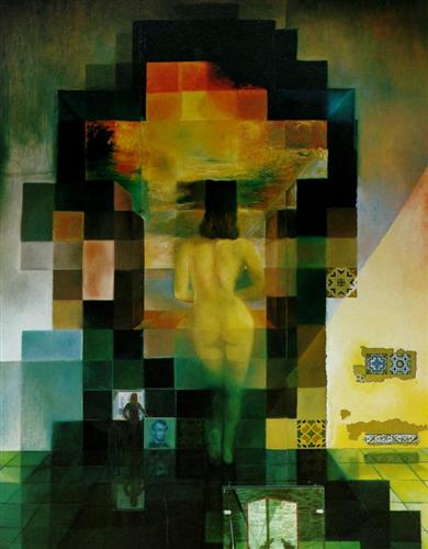
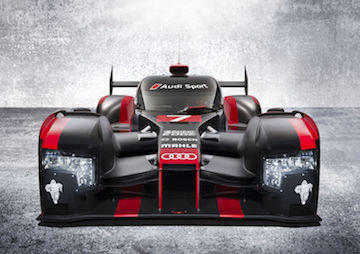
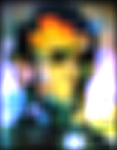
Original image
Original image: Licoln

Gaussian stack: sigma = 2

Gaussian stack: sigma = 4
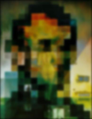
Gaussian stack: sigma = 8
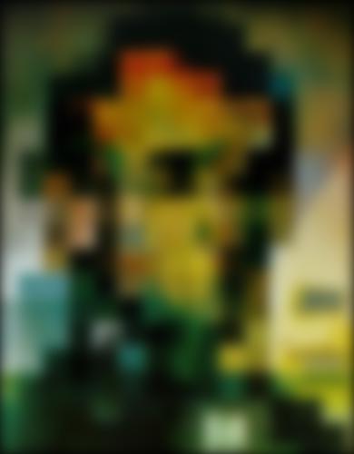
Gaussian stack: sigma = 16
Gaussian stack: sigma = 32
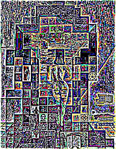
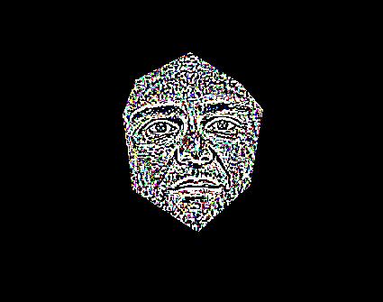
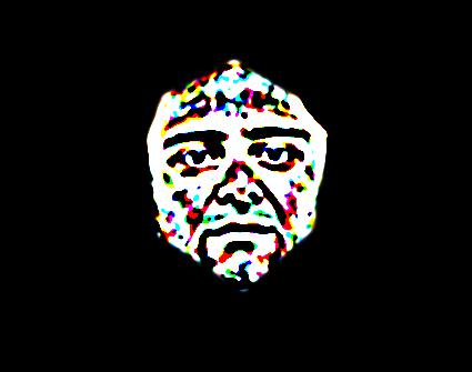
Laplacian stack: 1-2
Laplacian stack: 2-4
Laplacian stack: 4-8
Laplacian stack: 8-16
Laplacian stack: 16-32
Laplacian stack: Remains
Part 1.4 Multiresolution Blending:
All images are processed with 45x45 Gaussian filter, with sigmas = [1, 2, 4, 8, 16]
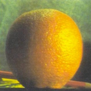
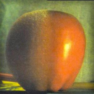
Original image: Orange
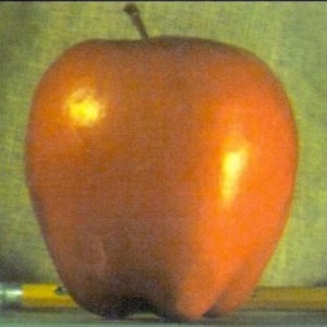
Original image: Apple
Blended: Oraple
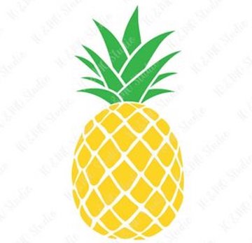
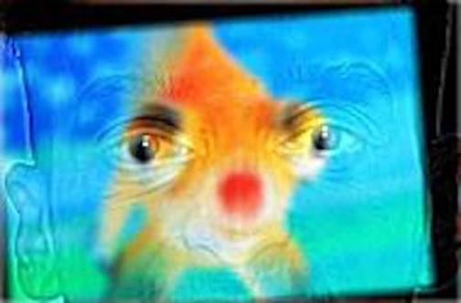
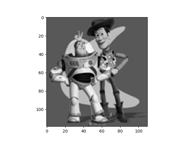
Original image: Pinapple Cartoon
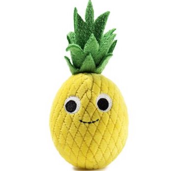
Original image: Pinapple Toy
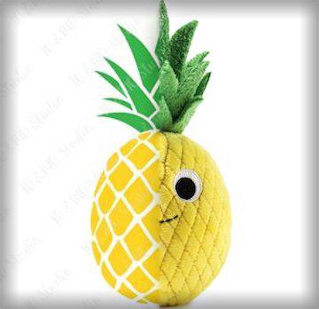
Blended: Pinapple Cartoy
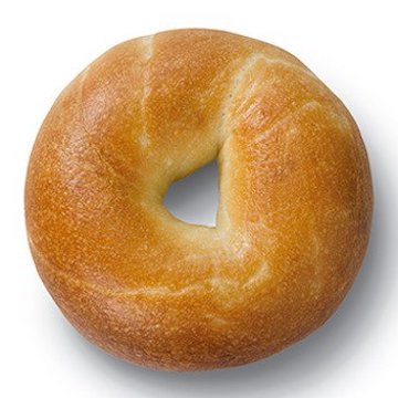
Original image: Bagel
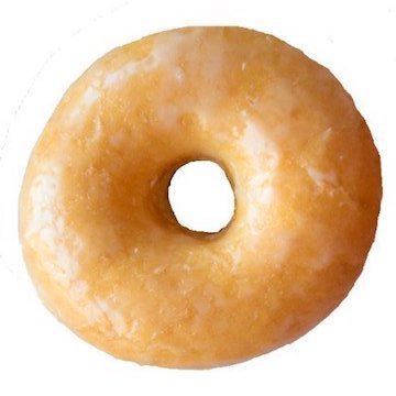
Original image: Donut
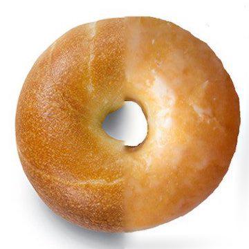
Blended: Bagnut
Failed case:
If the two object does not mesh well, horizontal/vertical blend fails
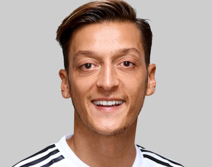
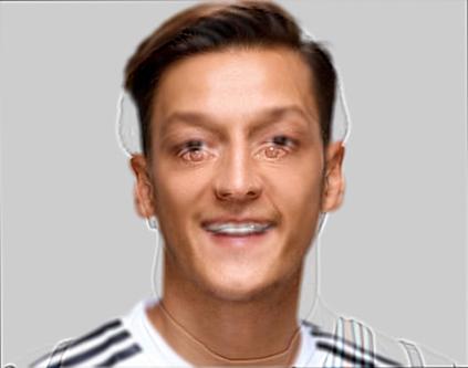
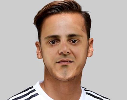
Original image: Ozil
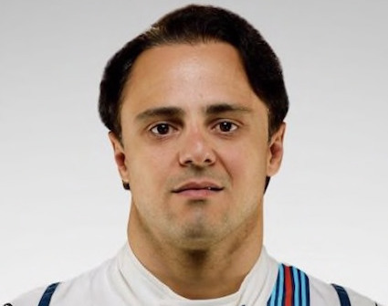
Original image: Massa
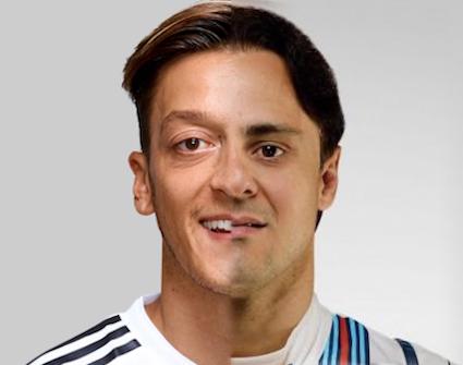
Blended: Failed?????
Solution: custom mask!!!!
So a custom mask is created to exploit the features of Massa

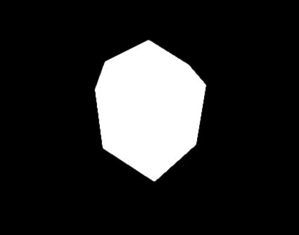
Custom Mask
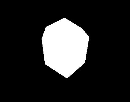
Original mask
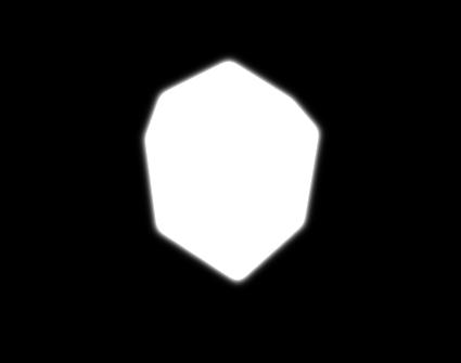
Gaussian stack: sigma = 1

Gaussian stack: sigma = 2
Gaussian stack: sigma = 4
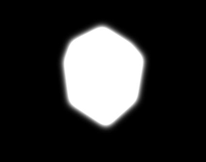
Gaussian stack: sigma = 8
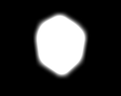
Gaussian stack: sigma = 16
Laplacian stack 0-1
Laplacian stack 1-2
Laplacian stack 2-4
Laplacian stack 4-8
Laplacian stack 8-16
Remains
Laplacian stack 0-1

Laplacian stack 1-2
Laplacian stack 2-4
Laplacian stack 4-8
Laplacian stack 8-16
Remains
Laplacian stack 0-1
Laplacian stack 1-2
Laplacian stack 2-4
Laplacian stack 4-8
aplacian stack 8-16

Remains
The final reveal:
Blended: Mazil
Bells and Whistles
The color is used to enhance the effect
Part 2.1 Toy Problem:
I constructed the A matrix and b vector using the idea of the MATLAB starter code in instruction: I accounted for all the horizontal constraints, then all the vertical constraints, and lastly matching the top left corner. This method is a bit a bit inefficient, because A is initialized to a full matrix, and entries are filled in by indexing. However, since the image is small enough, it did not take too long.
Due to the way I construct the matrix A, I had a hard time using the sparse matrix solver. In the end I just used a least square formula from CS189 to solve the Av = b equation: v = (A^T A)^{-1} (A^T b). The computation took about 15 seconds on my computer
It is worth noting that only when I put in cmap=cm.gray as an argument to imshow, the image displayed correctly. Othewise it displayed only in the blue channel
The result:
Output of the toy problem
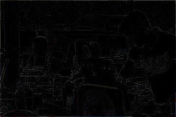
Part 2.2 Poisson Blending:
This is the constraints for Possion Blending:

I encode the constraints in my matrices by following the structure of the formula: breaking it down to constraints within the source images (first summation), and the constraints on the boarder (second summation). I break down each of the summation even more by separating horizontal constraints from vertical constraints. In the end, I basically have four parts that sum up to the objective: intra-horizontal, intra-vertical, inter-horizontal, inter-vertical.
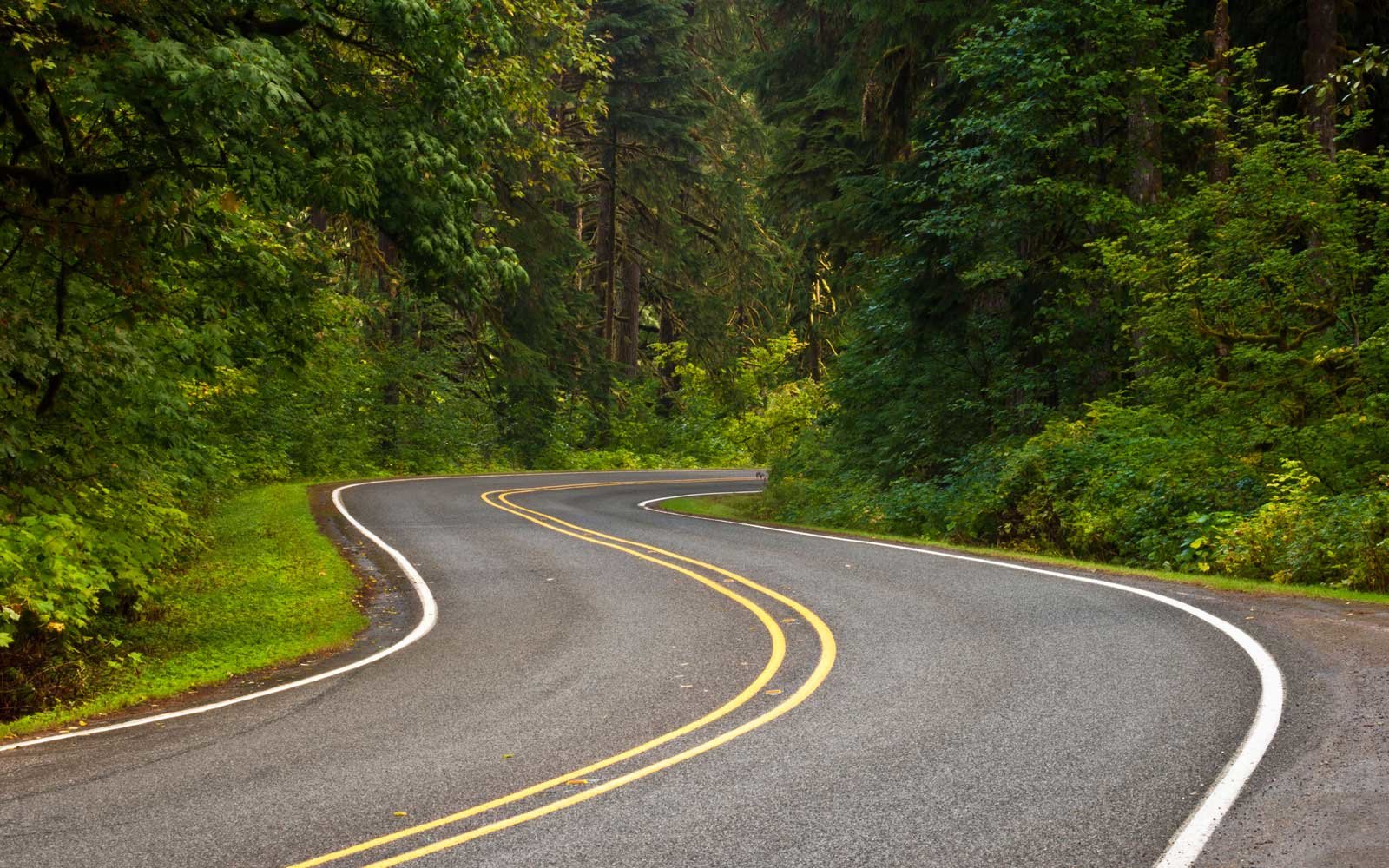
Original image: Mountain Road
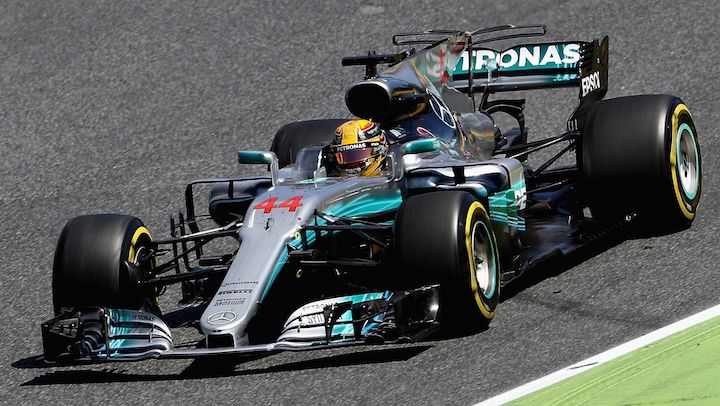
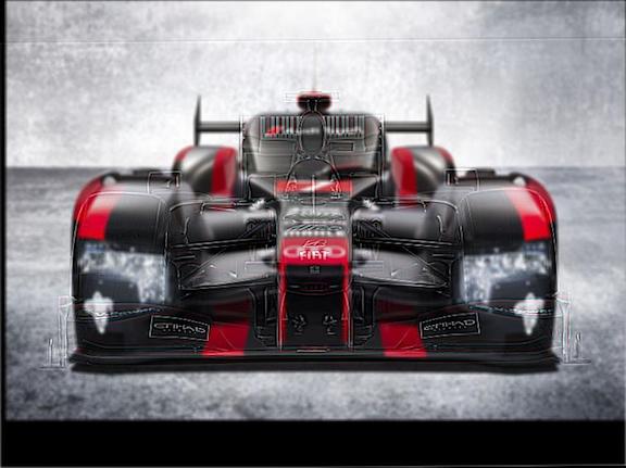
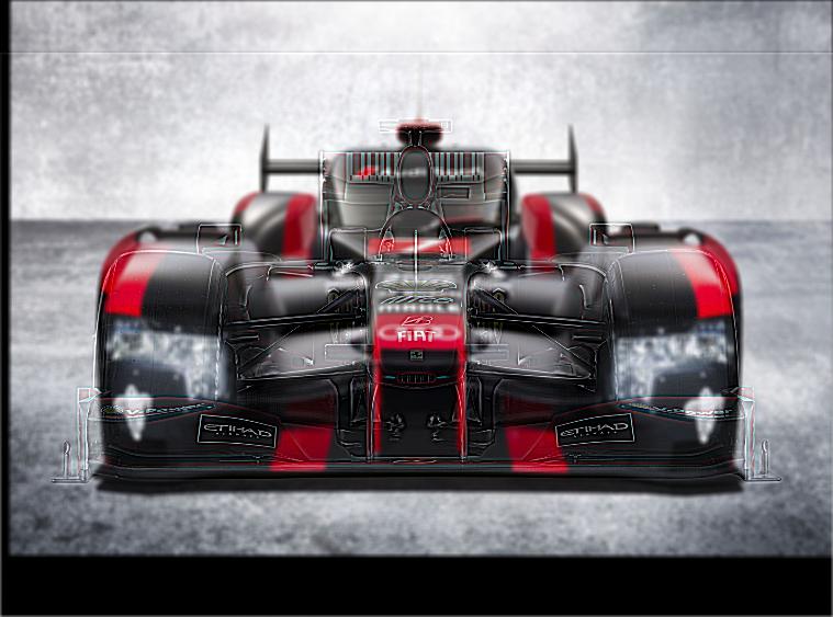
Original image: Mercedes F1
Mask for Mountain Road
Mask for Mercedes F1
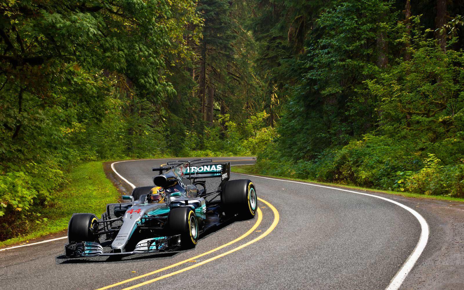
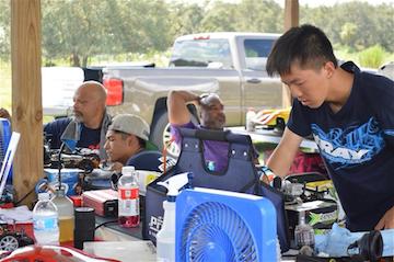
Direct Copy
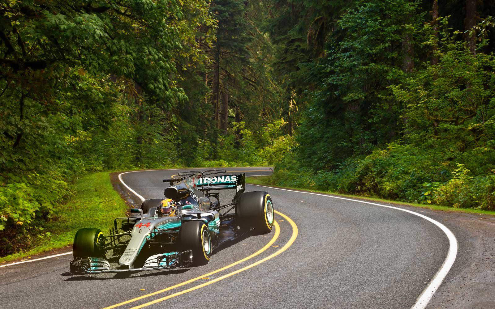
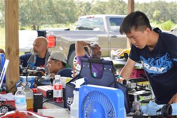
Result of Possion Blending
Although the direct copy on the left seems to have higher resolution, there are actually serious issue if we zoom in on the boarder of the car
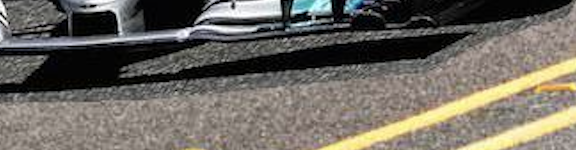
Direct Copy, zoomed: the separation between racetrack and road is very apparanent
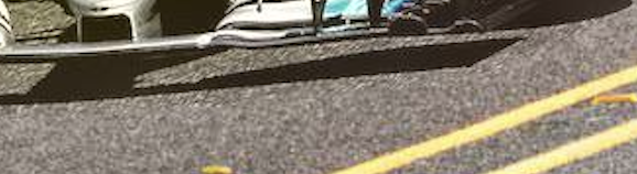
Possion Blending, the racetrack blends into the road perfectly
The Possion Blending version looks less "correct" overall because the difference between the background of the F1 car (black asphalt) and the mountain road, which can be understood as errors, are spread across the whole F1 car image
Extra images:

Original image: Berkeley
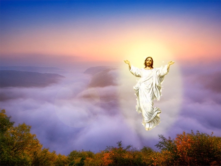
Original image: Jesus
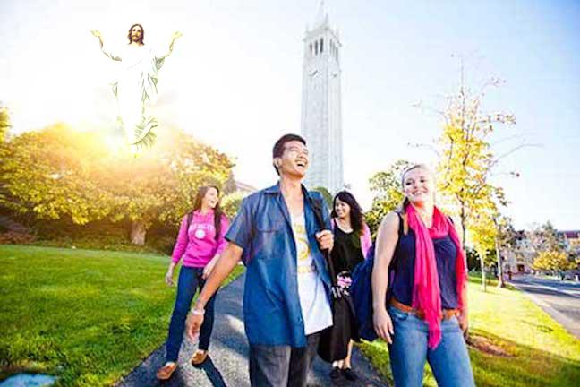
Blended: Jesus risen from Berkeley
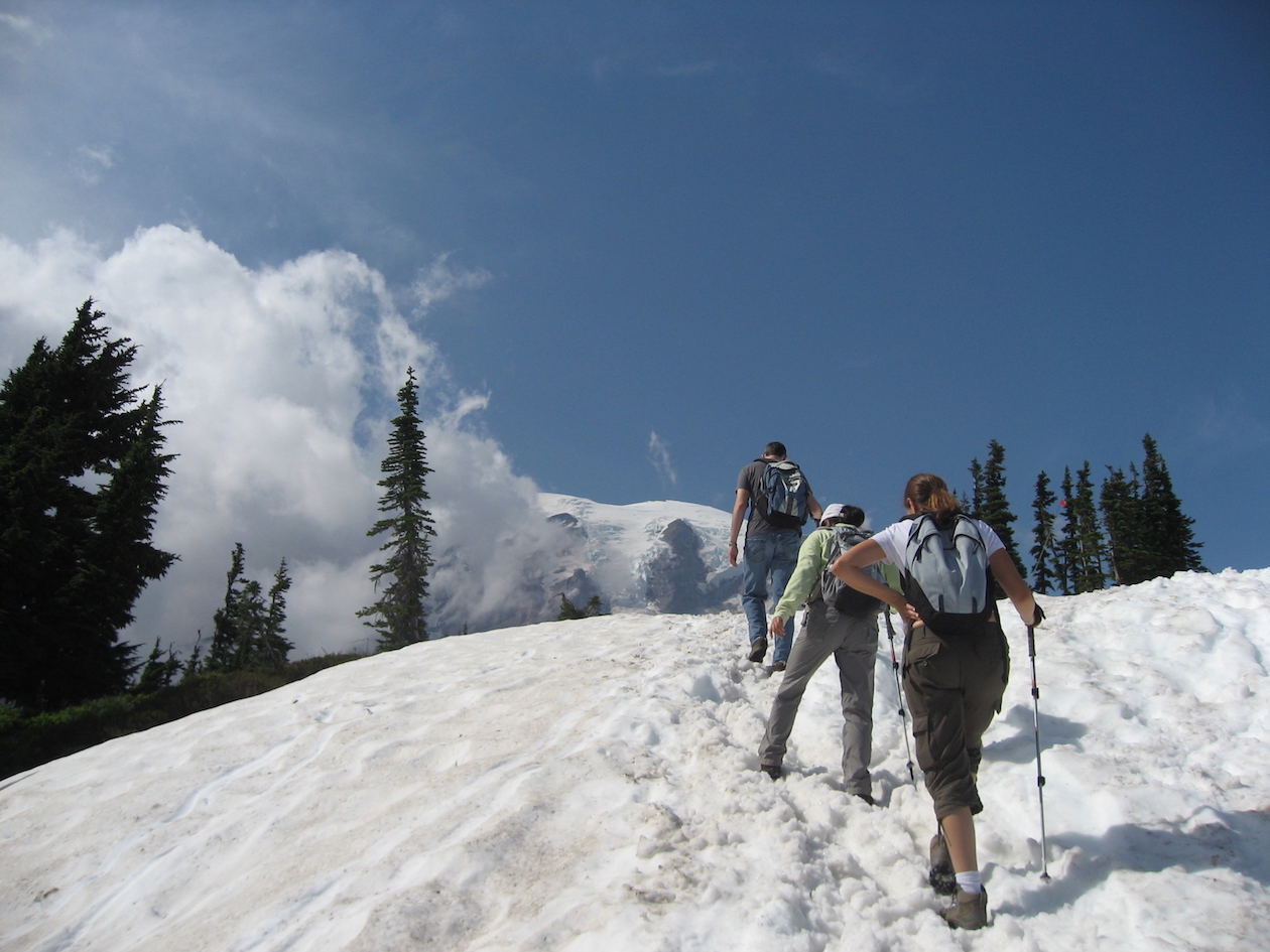
Original image: im3
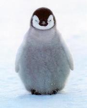
Original image: penguin chick
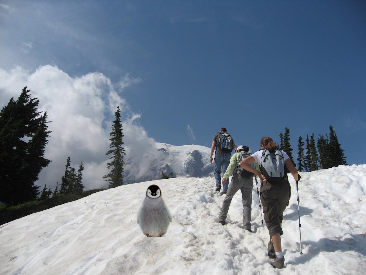
Blended: Penguin chick in the wild
Failed Case:
Original image: Mountain Road
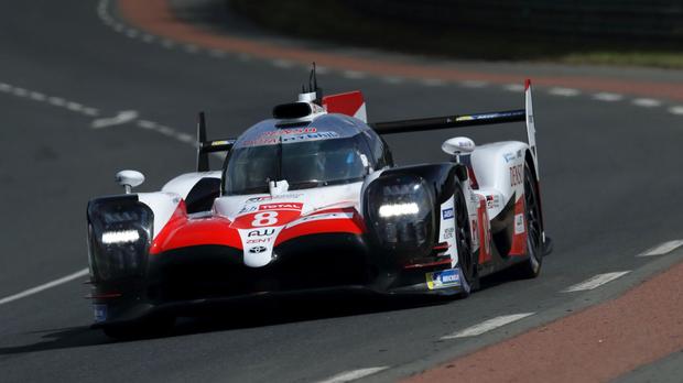
Original image: LMP1
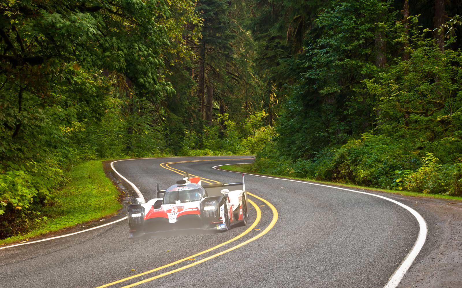
Blended: LMP1 on Mountain Road
This case fail because the background of the car (boarders of the selected region) is way too different from the mountain road. The error is so big that when spread across the whole image, it is still very noticable
Comparing Multiresolution Blending and Gradient Blending:
Recall we were blending these two images with Multiresolution Blending in Part 1.4
Original image: Ozil
Original image: Massa
Using the same mask from Multiresolution Blending, I perform Poisson Blending for these two images
Multiresolution: Mazil
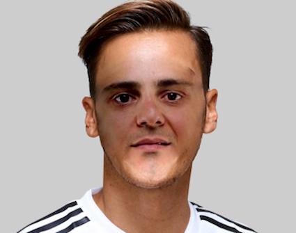
Poisson Blending: Mazil after his trip in California, where he wears wigs and fake beards
In this case, the Multiresolution work better because in the left side of the image, Possion Blending get screwed by Ozil's black hair, which is way too close to the masked region. I consider it "screw" because the hair near the boarder actually have no correlation with the face in the masked region.
Bells and Whistles: Mixed Gradient Blending
The Mixed Gradient is very interesting: it preseve the structre of the target image a lot more, and does not preseve the structure of the source image as much. In short, Mixed Grdient "blends in" the whole image a lot more.
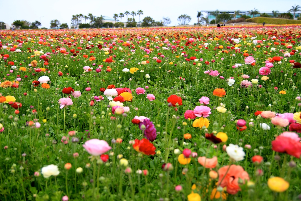
Original image: Flower Field
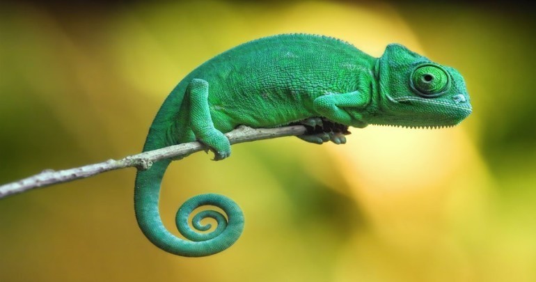
Original image: Chameleon
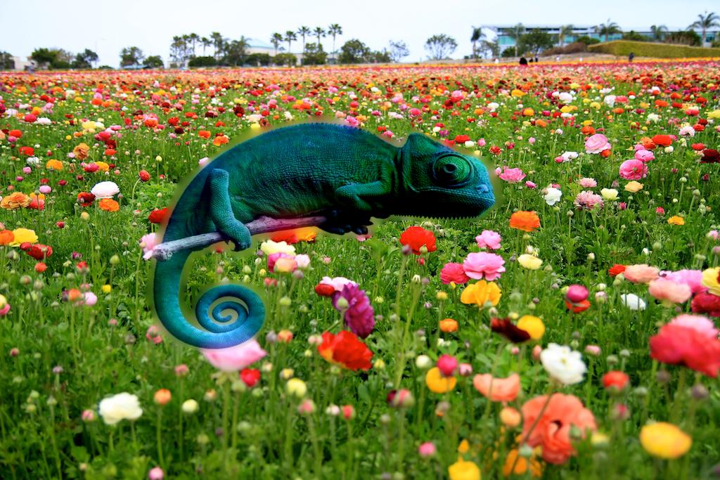
Poisson Blending
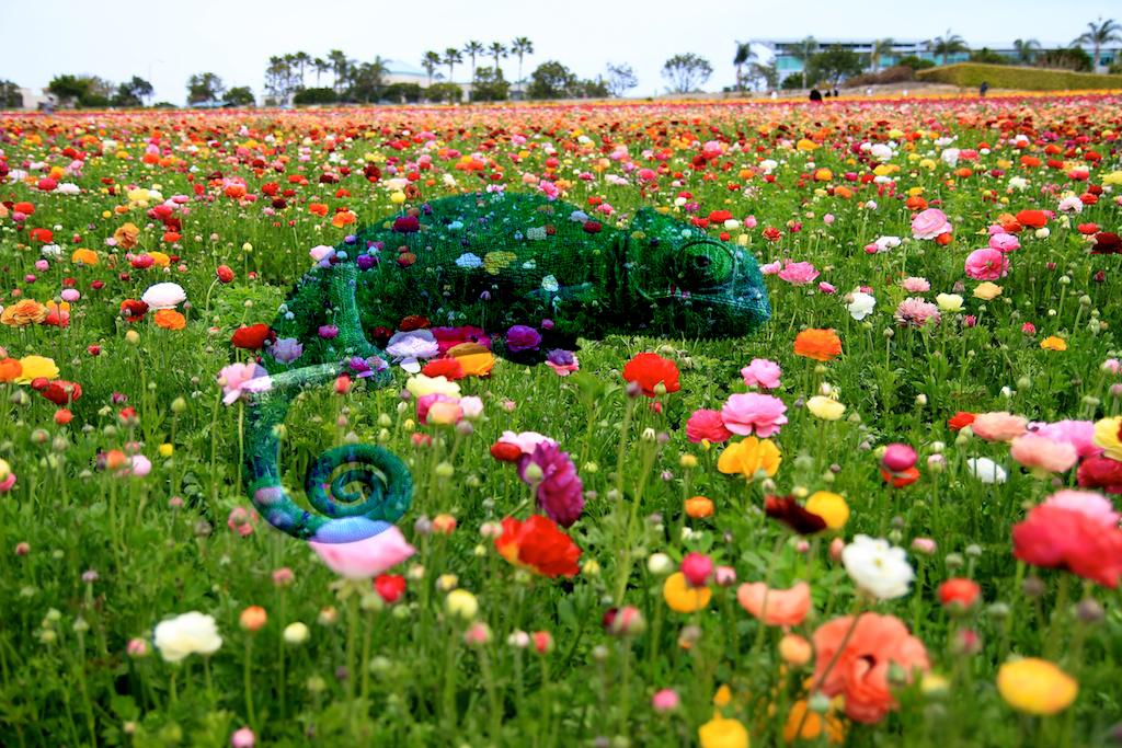
Mixed Gradient Blending: the Chameleon "blends in" a lot more