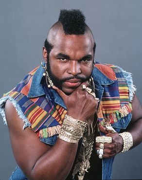
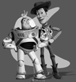
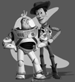
Mr T. looking pretty serious
|
 Mr T. looking not so serious
|
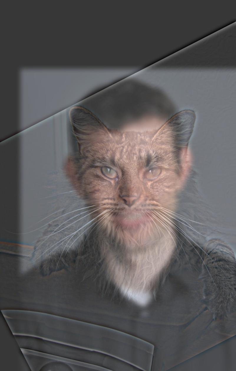
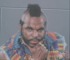 Hybrid of the two.
|
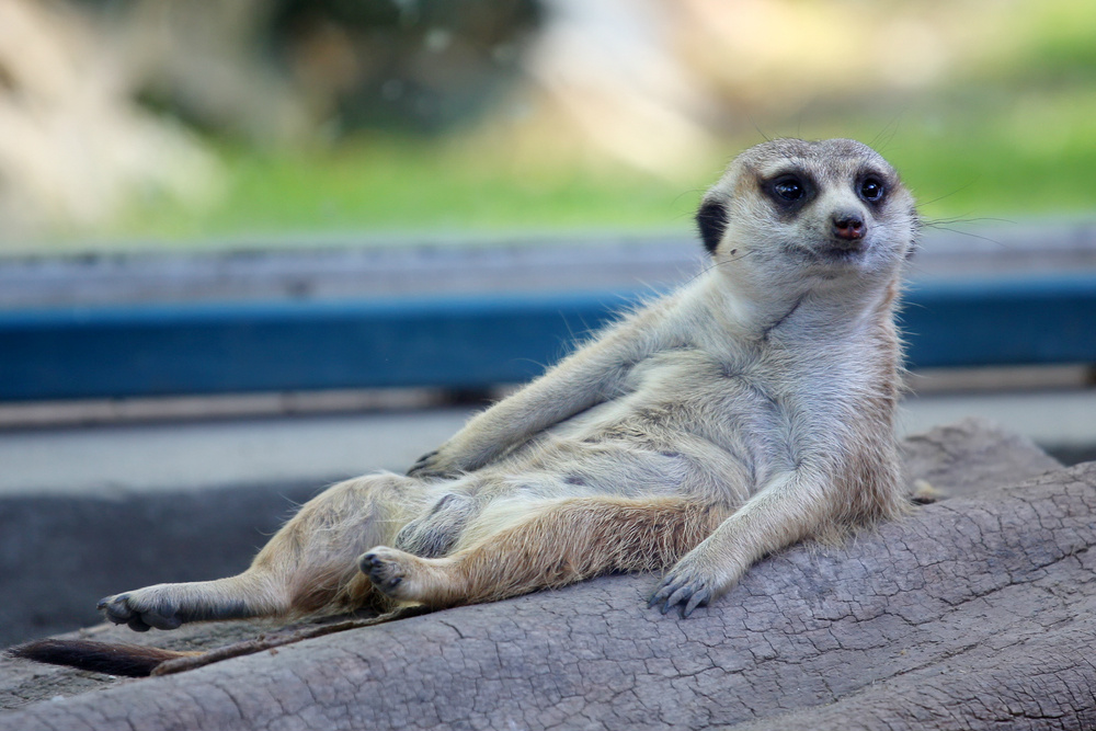
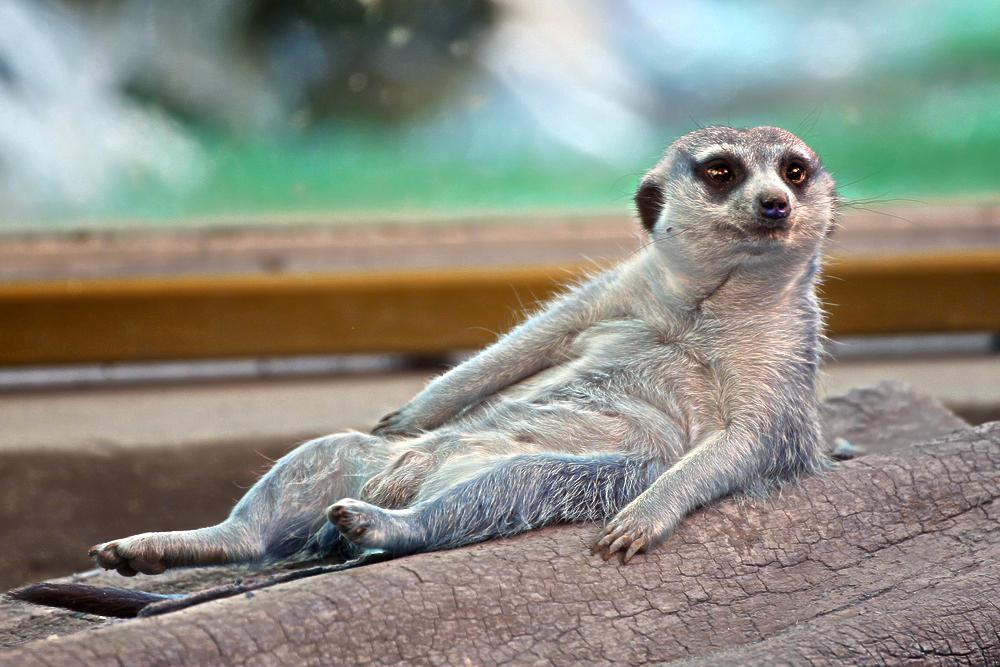
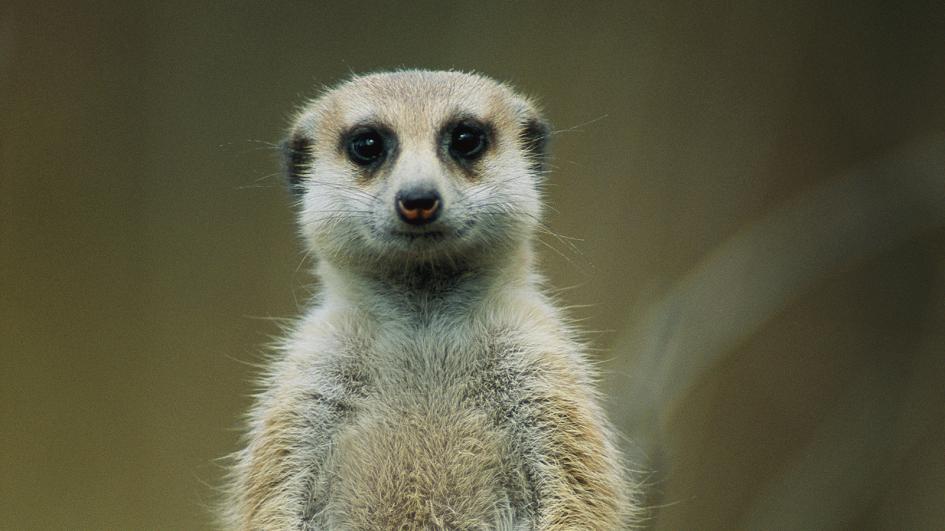 Picture of a meerkat
|
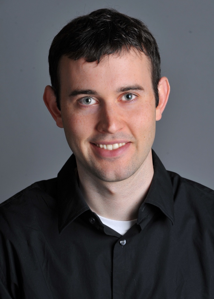
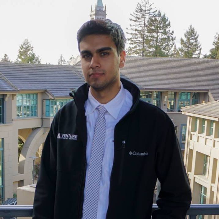 My roommate, who kind of looks like a meerkat
|
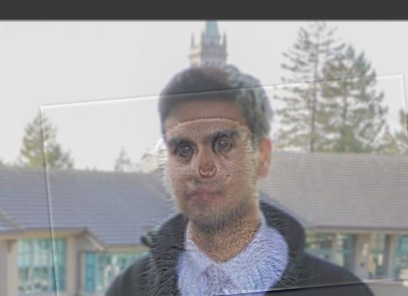 Hybrid of the two.
|
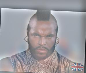
If you look closely at Mr T, he seems pretty serious, but if you look from afar, it seem like he's grinning! Here's a failed version that didn't go so well:
|
Mr T. looking pretty serious
|
Mr T. looking not so serious
|
 This one didn't turn out so well.
|
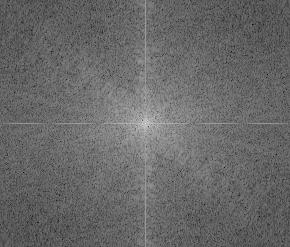
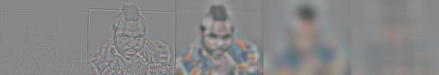
This failed image was most due to overtuning of the frequencies; I kept too many of the edge frequencies and too little of the blurred frequencies. Let's take a look at the frequency decomposition of the images:
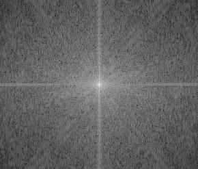 Freq Domain of Serious Mr T
|
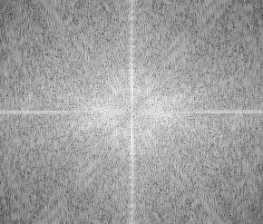
 Freq Domain of Not Serious Mr T
|
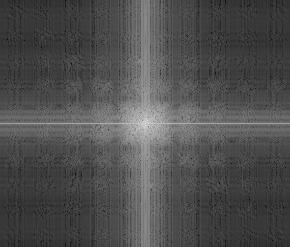
 Filtered of the above
|
 Filtered of the above
|
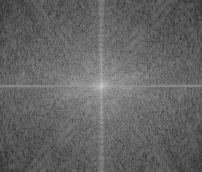 FFT of hybrid image
|
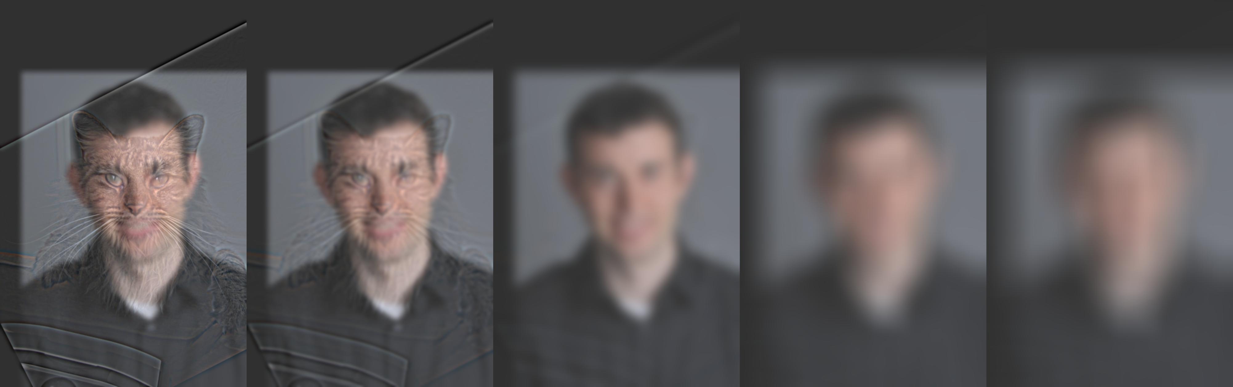
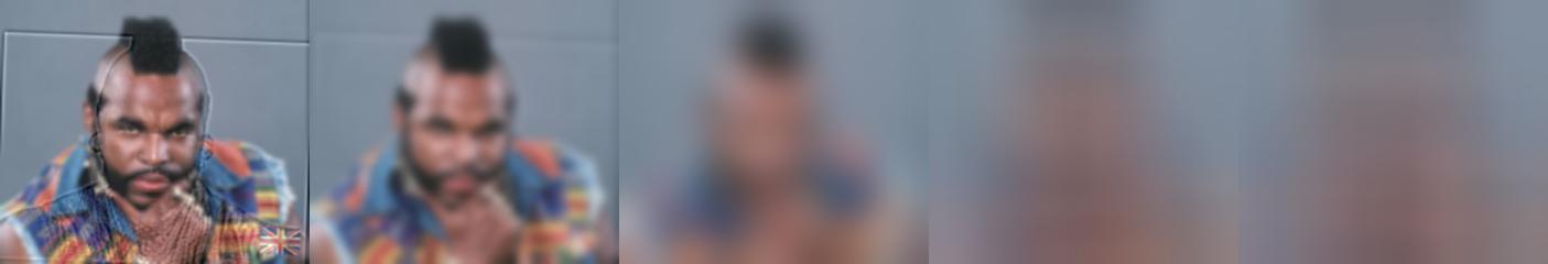
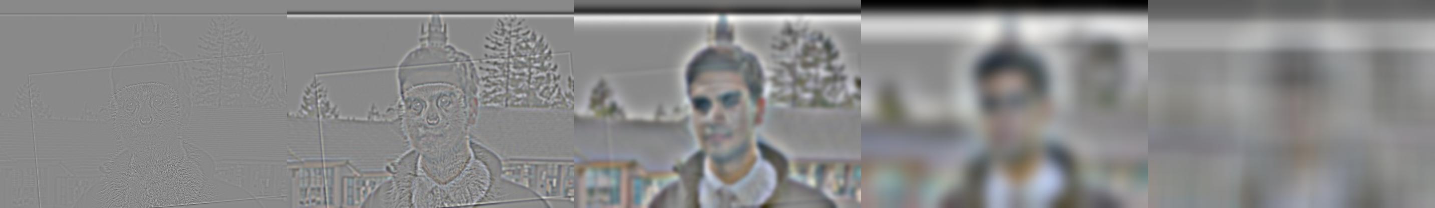
Part 1.3: Gaussian and Laplacian Stacks
In this section, we create gaussian stacks by repeatedly applying our gaussian filter to an image. We create a laplacian stack by taking the gaussian stack at level i, and subtracting it from the gaussian stack at level i - 1 (where level 0 is our original image). We can do some neat things with these stacks (as I'll show in the next part). Here are the gaussian stacks from some of the images in the previous part.
 Gaussian stack of sample hybrid
|
 Gaussian stack of Mr T hybrid
|
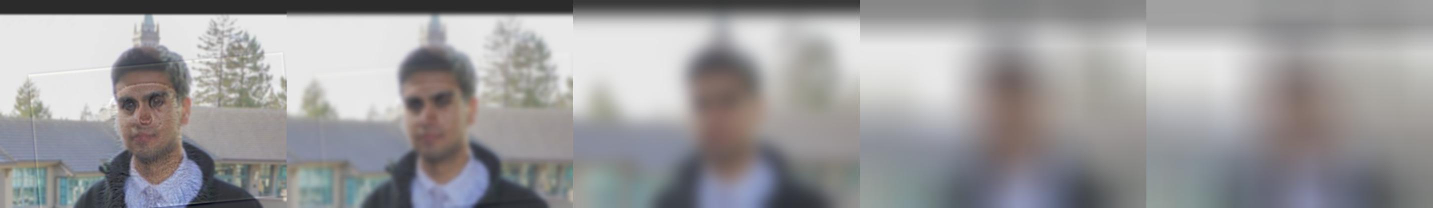 Gaussian of roommate + meerkat hybrid
|
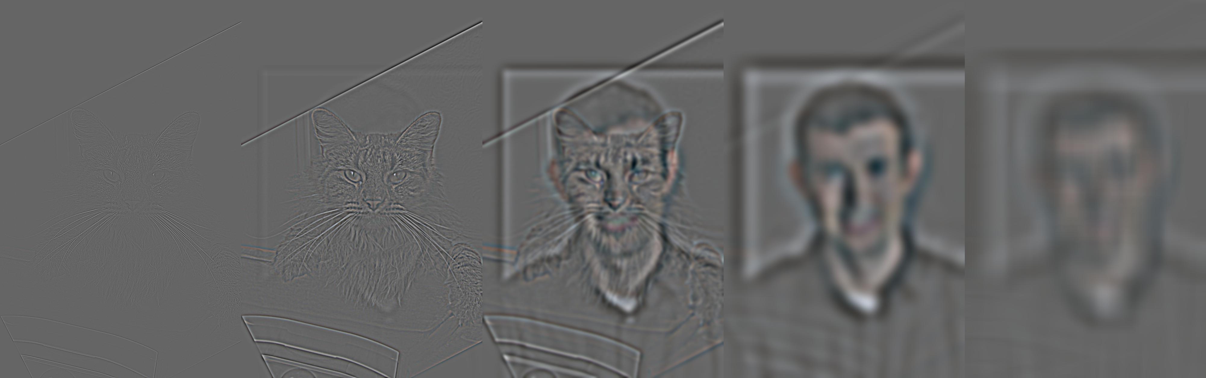
And the corresponding laplacian stacks:
 Laplacian stack of sample hybrid
|
 Laplacian stack of Mr T hybrid
|
 Laplacian of roommate + meerkat hybrid
|
Part 1.4: Multiresolution Blending
Using these gaussian and laplacian stacks, we can achieve a smooth blending effect between images. We start with a mask (1's where one image's pixels should be, 0's where the other image's pixels should be), and produce a gaussian stack of our mask. We multiply each level of our mask's gaussian with the gaussian of our two images (by a factor gaussian(mask)[i] for one image and 1-gaussian(mask)[i] for the other image) and in this way, match the "blur" of our mask with the "blur" of the contents we are trying to blend. Here are some examples:
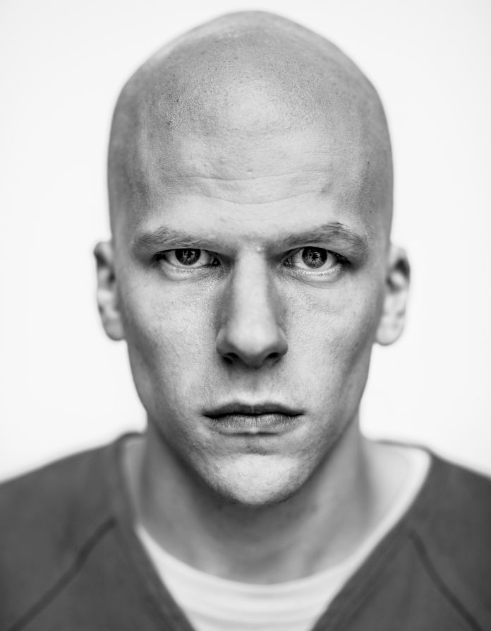 Jesse Eisenberg
|
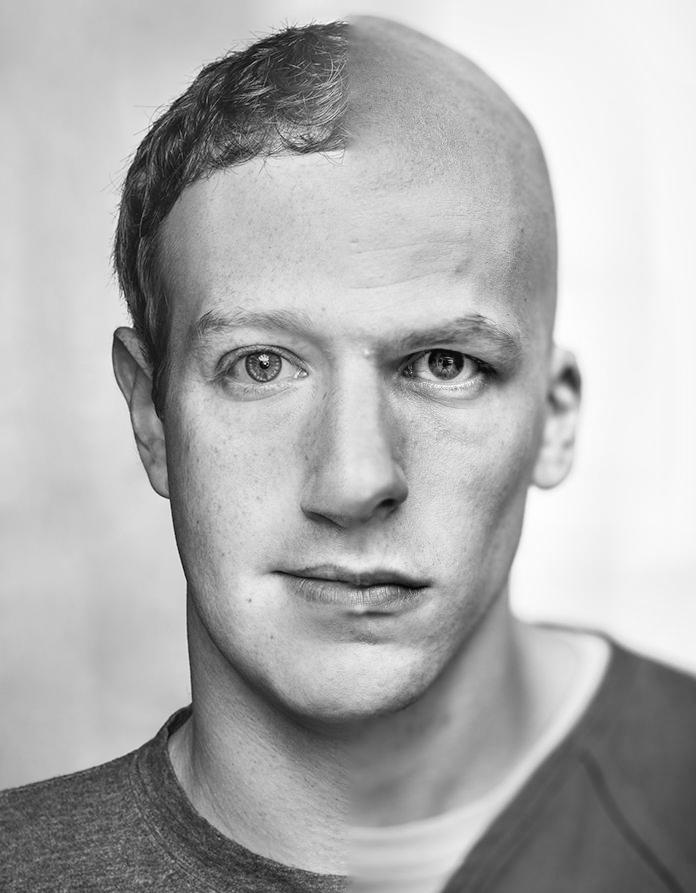
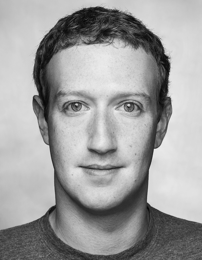 Mark Zuckerberg
|
 jesseberg?
|
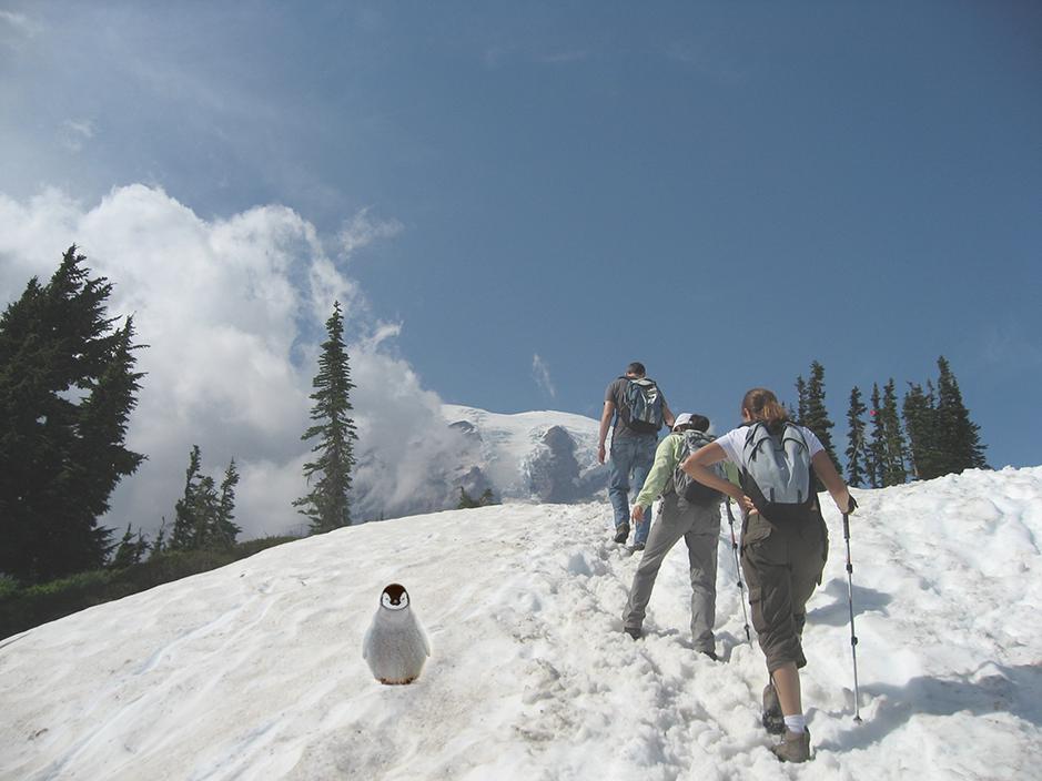
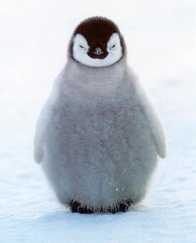 Penguin
|
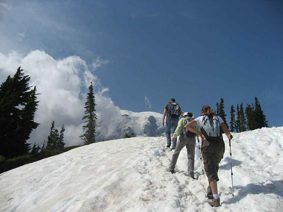 Sample photo
|
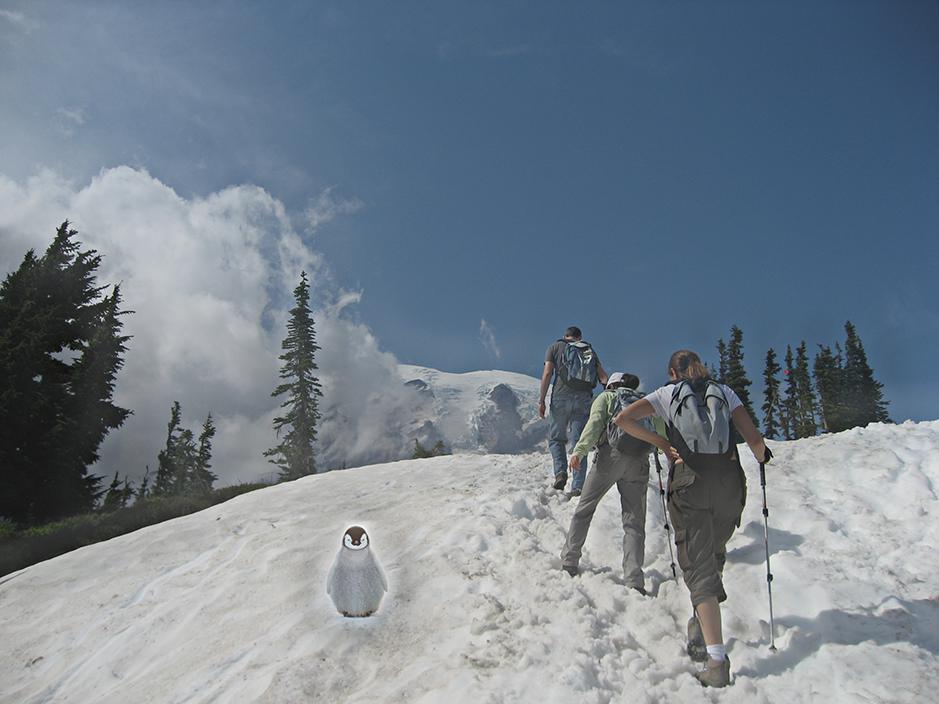 This doesn't work too well...
|
Part 2.1: Toy Example
In this section, we think about images in terms of their gradient domain. In blending images, we try to preserve the difference in values between pixels while trying to "match" the pixels where one image meets the other. This technique works well because humans are good at perceiving the differences between pixels, rather than the absolute pixel values themselves. In doing this, we try to optimize the following:
argmin_v(sum(((v_i - v_j) - (s_i - s_j))**2) + sum(((v_i - t_j) - (s_i - s_j))**2))
where i are all pixels in our mask, j is each adjacent neighbor pixel to x, s is our source image, t is our target image. To solve this complicated series of constraints, we can set up a least squares problem and "solve" for v to get a good optimization for our image.
As a quick proof of concept, we run this optimization on a single small "toy" image, and ensure that we are able to get back the same image after our algorithm runs. Since we aren't mixing the image with anything, we should expect to get back the same image.
 Original
|
 Result
|
Part 2.2: Poisson Blending
Now, we can apply this algorithm to blend images, here are the two images we'll be blending:
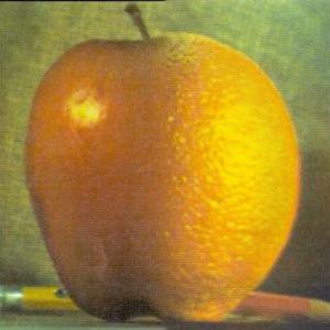
 Source Image
|
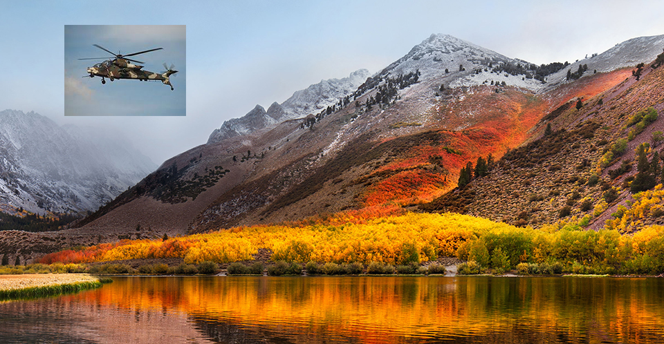
 Target Image
|
Here's how it looks if we simply copied the images from one to the other:
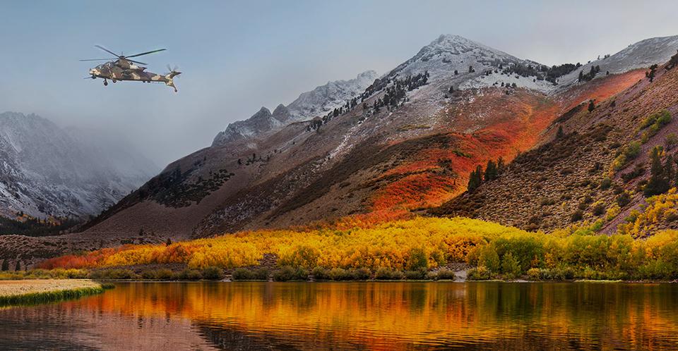
And here's the result of our poisson blending:
Other nifty poisson blends:
|
 This image didn't turn out too well; the source image is meant to be purple but looks green in the final render. This is probably due to the underlying boundary of the target photo being green and shifting the color of the pixels that were blended in.
|
Here's an image that I tried to blend originally with multiresolution blending. It didn't look good before, and I got startlingly better results with poisson blending. It seems that in this situation, poisson blending worked a lot better, but it didn't work well at all in other scenarios (that I forgot to save). I would commonly run into situations where the source image would take on the color characteristics of the target image, and the entire algorithm seems to only work well in situations where the boundary between the source and target are of somewhat similar colors, where multi-resolution blending doesn't run into that problem. However, in examples such as the one below, poisson blending is able to achieve much better results when operating within those conditions.
Bells and Whistles
Each of the parts have been implemented in color.