Part 1: Frequency Domain
Part 1.1: Unsharp Mask
Part 1.1: Unsharp Mask
The goal of this section was to produce an image sharpening effect using the technique we discussed in lecture. Since a Gaussian kernel convolved with an image returns the lower frequencies of said image, we can subtract these frequences from the original images to get the higher frequencies. We then add these higher frequencies back to the original image, making it look "sharper" because the higher frequencies have been amplified.
Mathematically, we can express this as:
image + alpha * (image - convolve(image, gaussian))
where alpha is a parameter scaling the intensity of the higher frequencies we're adding back.
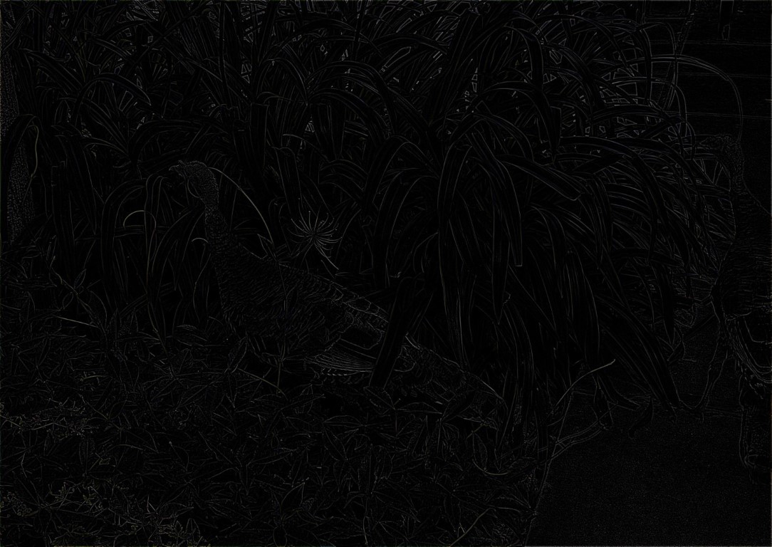
Below, we can see the unsharp masking process on a few images. It might
be a bit difficult to see that the images have been processed at all
at this size (especially for the "Higher Frequencies" column).
I highly recommend opening these images in a new tab to
see the details and the differences. The alpha used for all images is 0.5.
Original

bird.jpg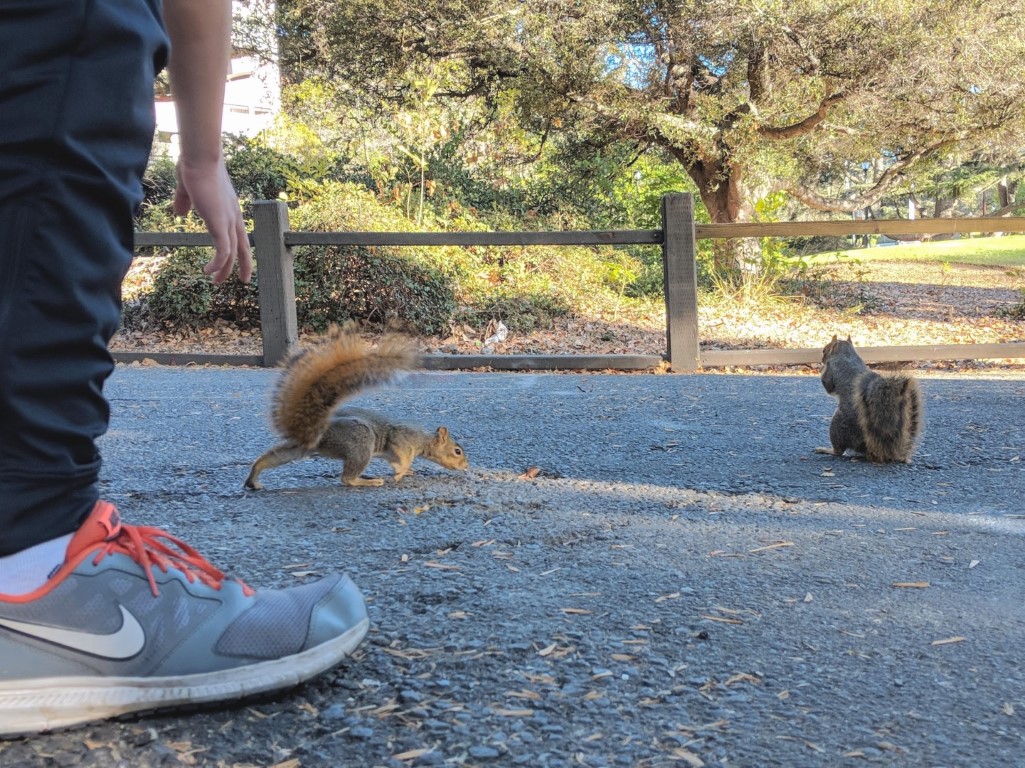
squirrel.jpg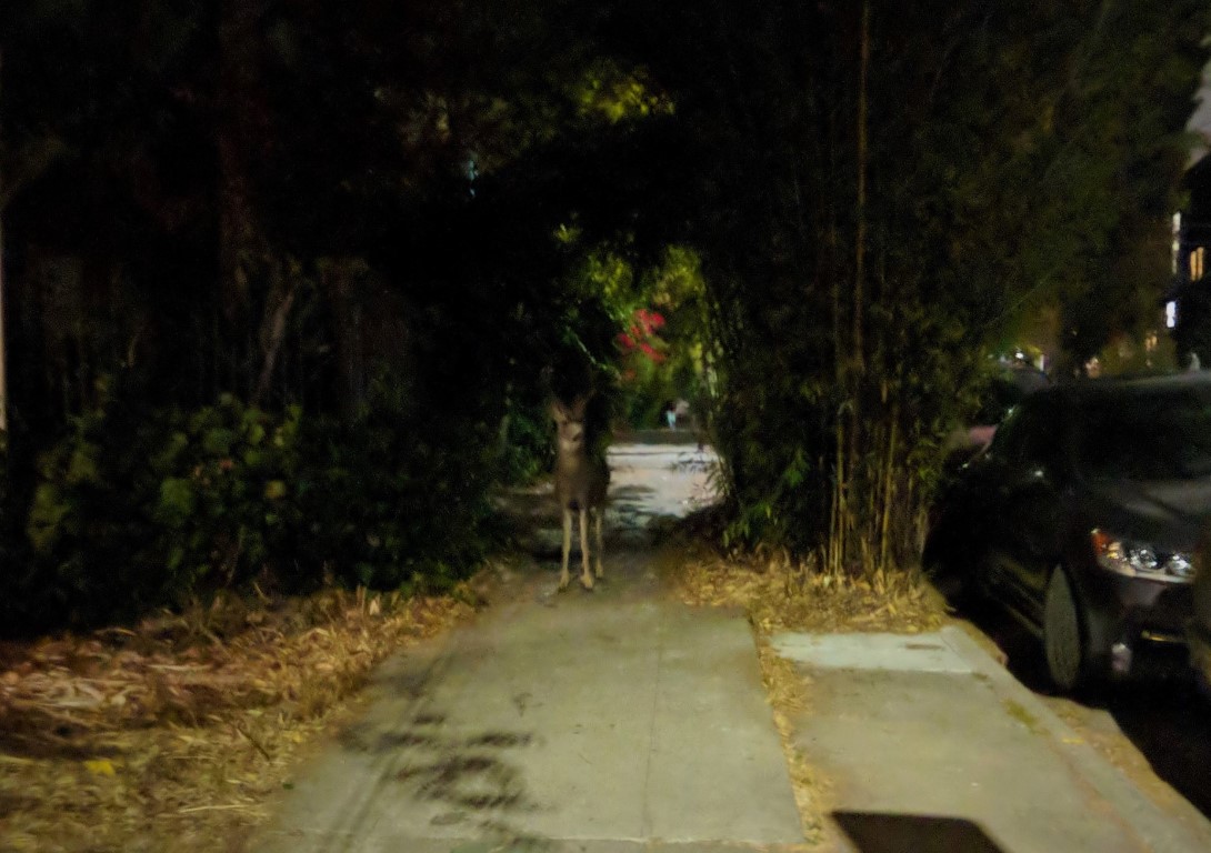
deer.jpgLower Frequencies
blurred-bird.jpg
blurred-squirrel.jpg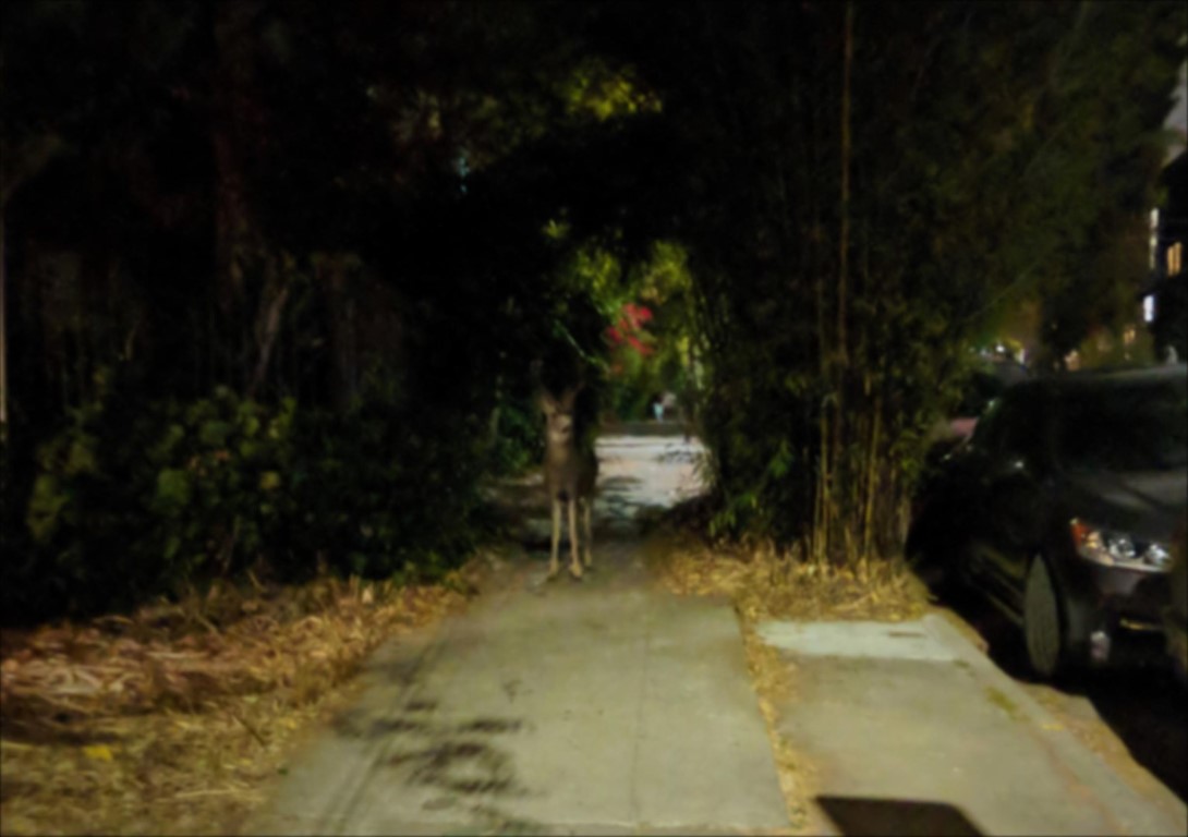
blurred-deer.jpgHigher Frequencies
detailed-bird.jpg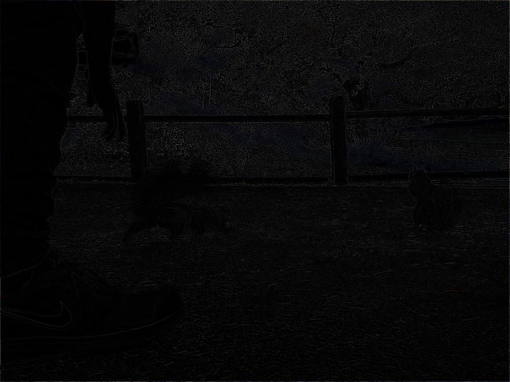
detailed-squirrel.jpg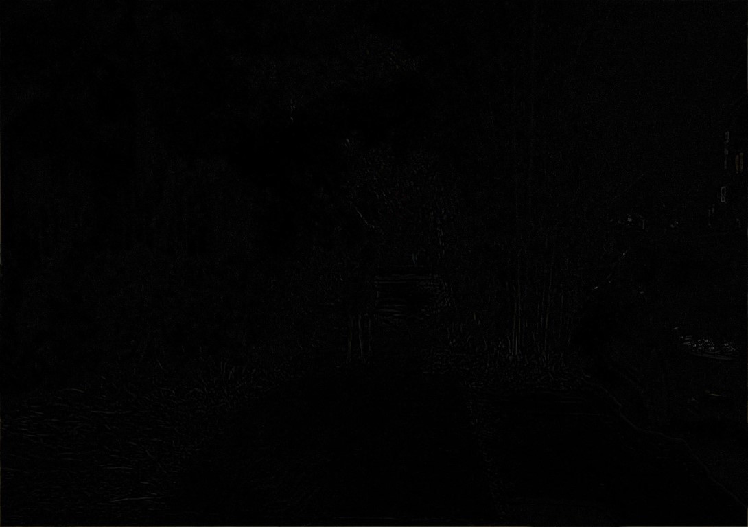
detailed-deer.jpgSharpened

sharpened-bird.jpg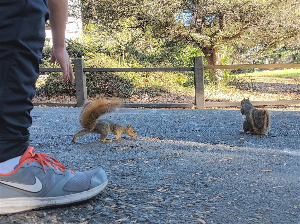
sharpened-squirrel.jpg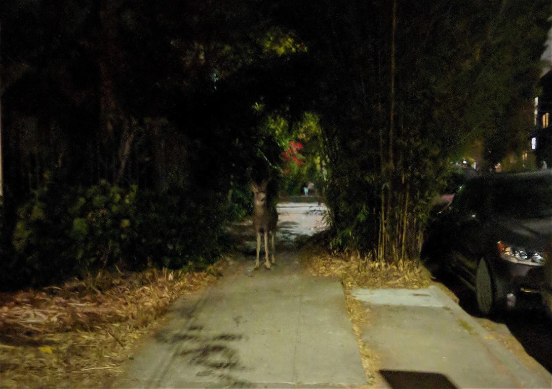
sharpened-deer.jpgPart 1.2: Hybrid Images
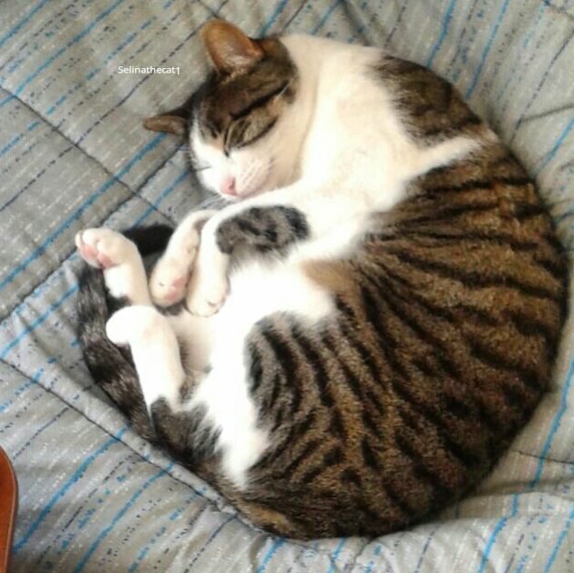
In this part, we attempt to create "hybrid images" by taking the high frequencies of one image and averaging them with the low frequencies of another image, using two different cutoff frequencies (i.e. two different sigmas to produce two different Gaussian kernels with differnet variances). Though this method manages to semi-merge two images, the effect is rather "ghosty" and isn't terribly convincing, however interesting. Nevertheless, let's see some fun examples!
Image 1 (High Frequencies)
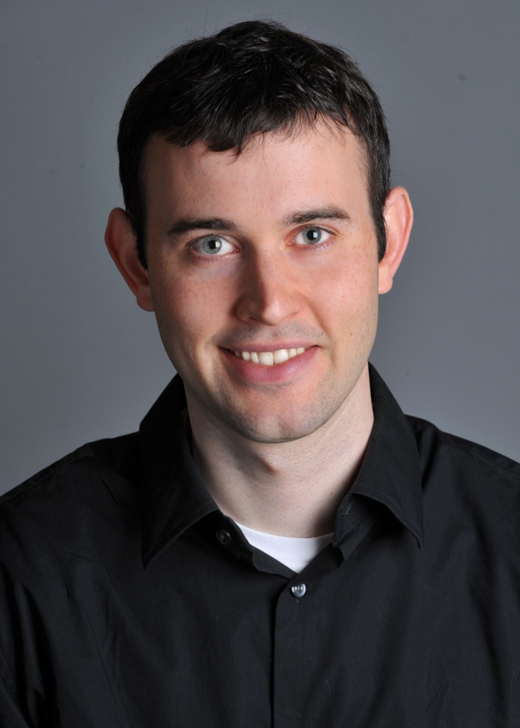
Image 2 (Low Frequencies)
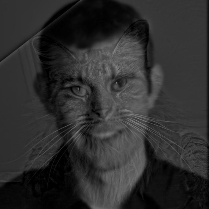
Hybrid Image
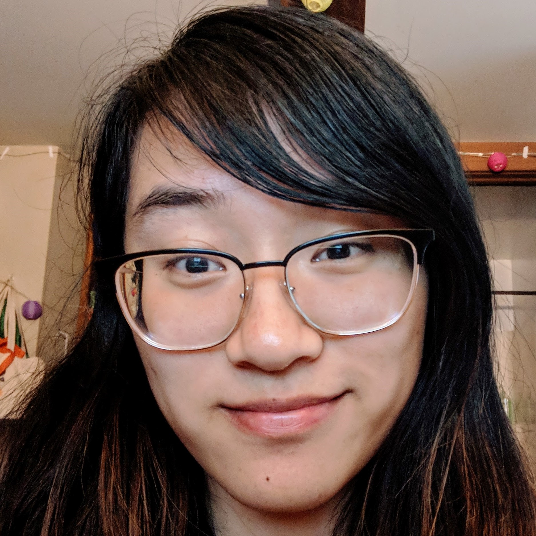
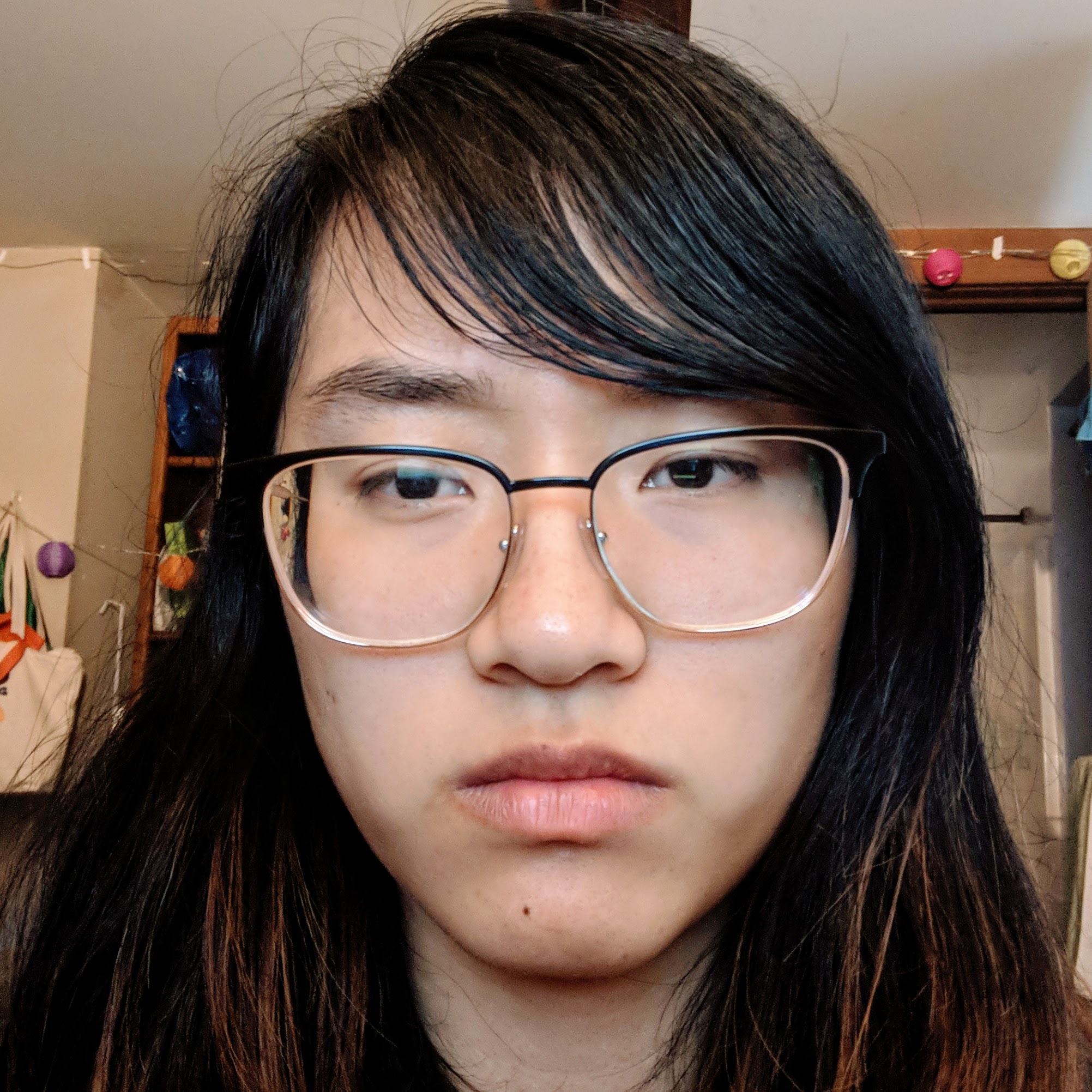
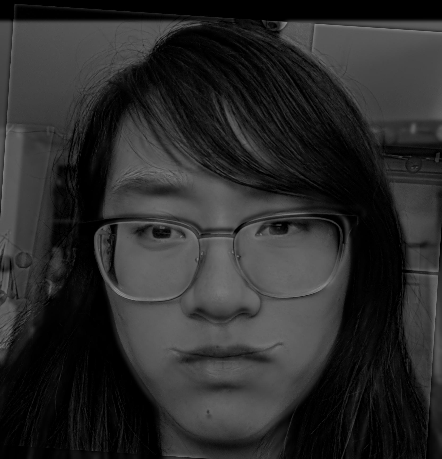
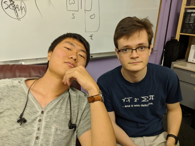
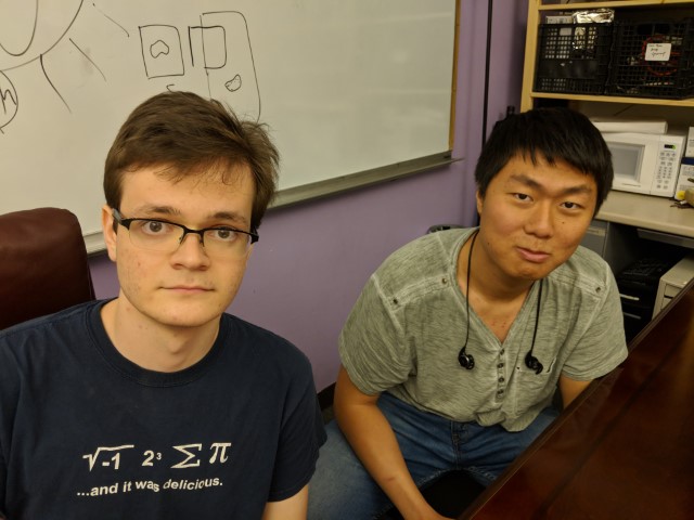
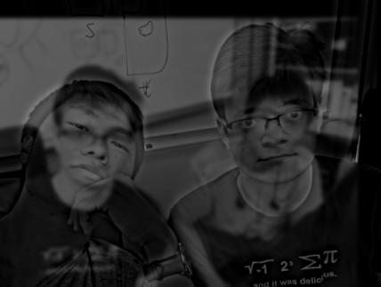
Note that "Nilbert and Gate" is a very obvious failure case. This is because, although I attempted to align these images via my friends' two noses, their poses are very different in each image, and their distance from the camera changes between images. As a result, we cannot get a workable alignment for these two images. Moreover, one of the most highest-frequency features in the first image is the formula written on Nate's blue shirt, causing it to be picked up and end up "hovering" oddly on the table in the hybrid image.
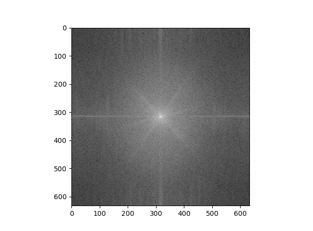
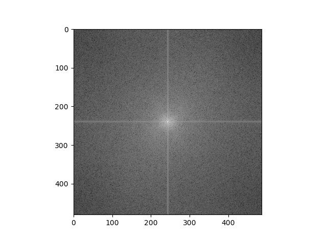
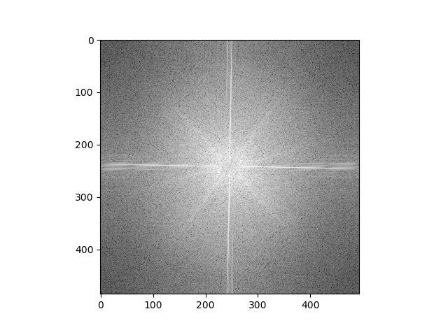
Now, let's examine the Fourier transforms of the "Catte" hybrid image:
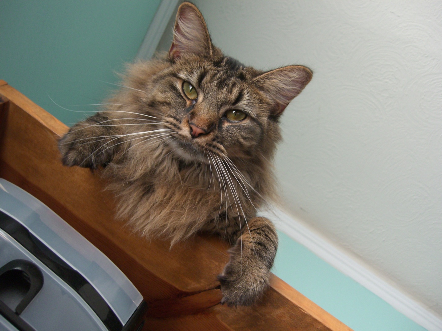
Cat, Input (High Frequencies)
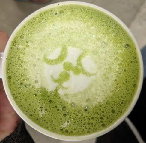
Matcha Latte, Input (Low Frequencies)
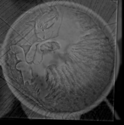
Cat, Filtered (High Frequencies)
Matcha, Filtered (Low Frequencies)
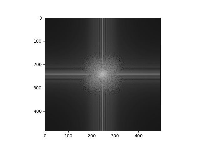
Hybrid Image
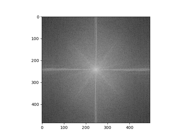
We can see that the plot is brighter (i.e. the magnitudes are higher) further away from the axes in the cat plot post-filtering, which makes sense, since we are grabbing the higher frequencies of the cat image via filtering. Similarly, the plot is brighter closer to the axes in the matcha plot post-filtering because we are trying to grab only the lower frequencies in that image. We then see frequencies of both plots in the hybrid plot - the "X" shape seen in the cat plot and the "+" shape seen in the matcha plot both show up in the hybrid plot, though neither shape is as bright as in their respective plots due to averaging.
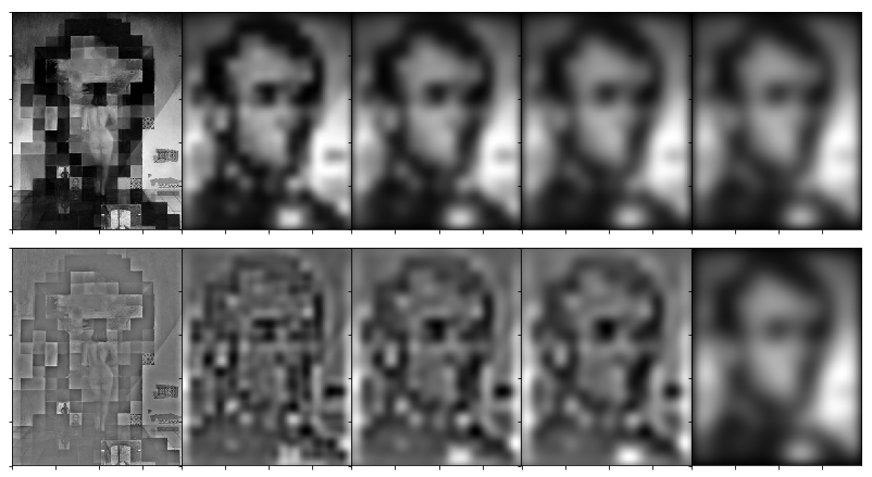
Part 1.3: Gaussian and Laplacian Stacks
In this part, we implemented Gaussian and Laplacian stacks - that is, ordered sets of images for which each "level" of the stack represents different frequencies. For a Gaussian stack, each successive level represents lower and lower frequences. For a Laplacian stack, each successive level represents a lower and lower band of frequencies - a Laplacian stack, in other words, breaks up an image into frequency bands such that - if you stacked all of the Laplacians on top of each other, we would get the original image back.
To implement the Gaussian stack, we repeatedly convolve the same Gaussian kernel
with the last Gaussian-convolved image. That is, a level i
image is the level i-1 image convolved with a Gaussian kernel.
To implement the Laplacian stack, we subtract pairs of images inside the Gaussian stack - this gives us the "band" of frequecies we're looking for, because with each application of the Gaussian kernel, more and more "high" frequencies are removed. Subtracting between pairs gives us the band of frequencies that was removed. The last image in a Laplacian stack is always the last image in the corresponding Gaussian stack, since that Gaussian represents the lowest band of frequences in the stack and thus enables us to reconstruct the original image by layering all the Laplacians on top of each other.
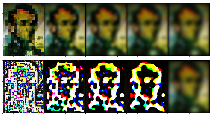
Let us use the Salvador Dali painting of Lincoln and Gala to examine these ideas! Note how each level of the Gaussian stack is blurrier than the previous, and how each level of the Laplacian stack shows a different set of details than the previous.
Original
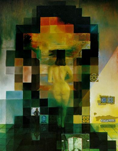
Grayscale
Color
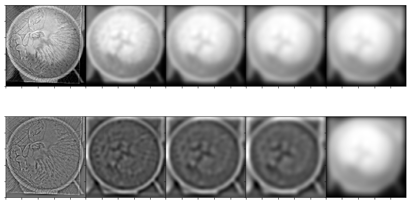
Now, let's examine the construction of one of our hybrid images, "Catte" - we can see about where both the "low frequency" and "high frequency" images start to show up. The latte becomes more and more obvious in the Gaussian stack, and the cat disappears quickly in the Laplacian stack.
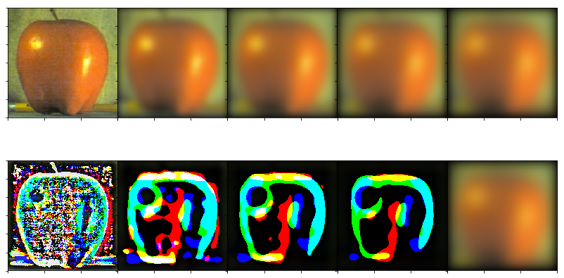
Part 1.4: Multiresolution Blending
In this part, we create image splines via multiresolution blending! We use different (frequency) resolutions of two images (using our Gaussian and Laplacian stacks) as well as different resolutions of a (initially) binary mask. What this does, is blend the two images smoothly across multiple frequency bands, as opposed to just splicing the two images together with the hard seam that simply applying the binary mask would cause.
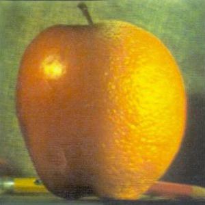
In order to achieve the blended "Orapple" below, we use the following Gaussian and Laplacian stacks as well as the following formula:
for i in range(numberOfLevels):
  final += gaussian_mask[i+1] * laplacian_img1[i] +
        (1-gaussian_mask[i+1]) * laplacian_img2[i]
where i represents the current level of the stack,
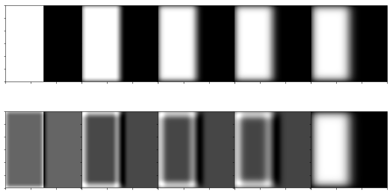
gaussian_mask represents the Gaussian stack of the binary mask,
and laplacian_img1 and laplacian_img2
represent the Laplacian stacks of source Image 1 and source Image 2
respectively. In other words, we combine shared frequency bands using a
blurred mask, then create a final blended image by adding up all of
these combinations. It is exactly because we're blending similar frequencies
smoothly, that we achieve this overall smooth seam.
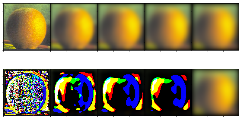
"Orapple"
Apple
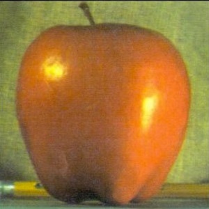
Orange
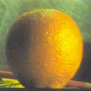
Blended
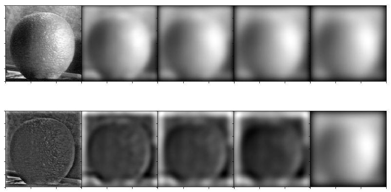
Apple Stacks
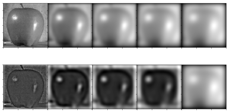
Orange Stacks
Mask Stacks
Apple Stacks in Color
Orange Stacks in Color
Mask Stacks in Color
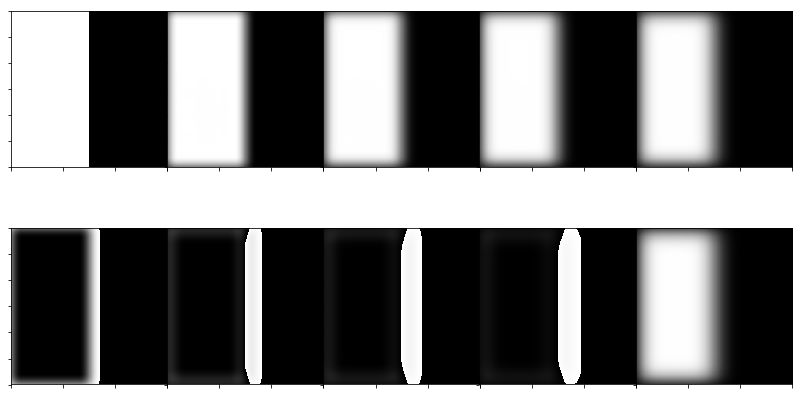
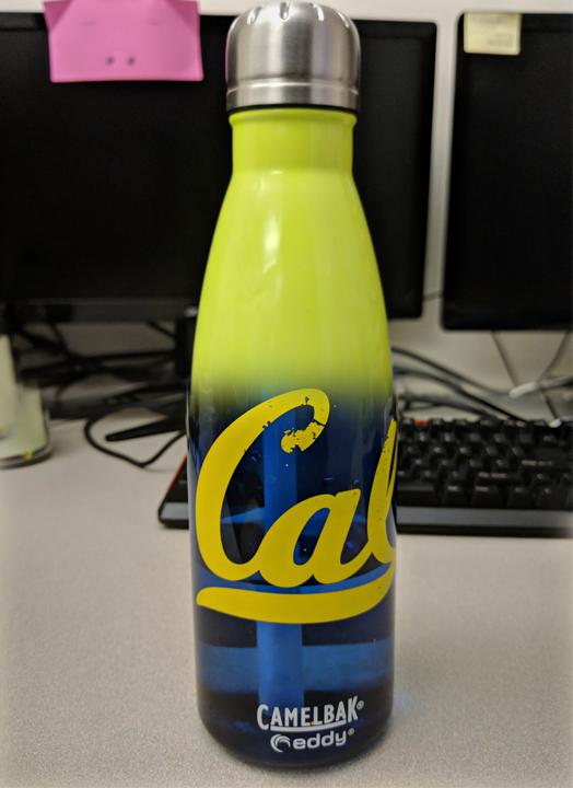
Here is another example, this time blended horizontally (i.e. binary mask is split directly in half)! What a neat water bottle... I wish I had one like that.
"Cool Water Bottle"
Blue Bottle

Green Bottle
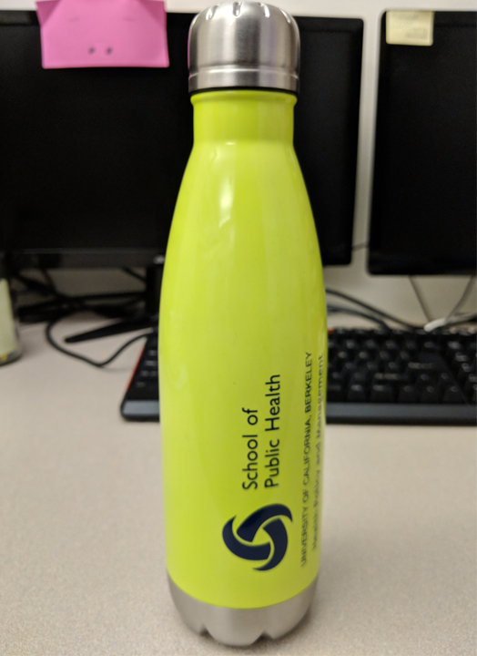
Blended
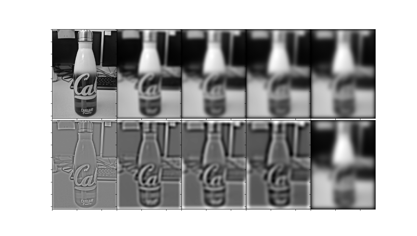
We can examine the Gaussian and Laplacian stacks for this one to see how the frequency bands blend together at each level:
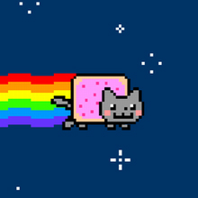
Now let's try it with an irregular mask!
"Space Cat"
Part 2: Gradient Domain Fusion
Part 2: Overview
Part 2: Overview
The goal of this part of the project is to use Poisson blending to map a source image into a target image smoothly - in a way that blends the source relatively seamlessly into the background of the target image - by minimizing the differences between the boundary gradients between the source and target images while also minimizing the differences among internal gradients (both in the x- and y-directions) inside the source image.
Part 2.1: Toy Problem
In this part, we test our understanding of how to solve the optimization problem entailed by Poisson blending by formulating least squares. We try to reproduce the gradients of the image on the left by finding pixel values that minimize the difference between our solution's gradients and the left image's. In other words, we want to reconstruct exactly the image on the left, making the gradients are the same. However, we must add one other constraint, which is that the top-left corner pixel of our reconstructed image must be the same as the top-left corner pixel of the original image. Otherwise, there could be many other solutions with similar gradients but not the same absolute pixel values.
After we construct a sparse matrix A and a vector of
constants b and solve,
this is the result! The image on the left is the original; the image on
the right is the reconstruction.

Part 2.2: Poisson Blending
In this part, we expand past the toy problem and actually try to blend a source image into a target background image. We expand the optimization problem: rather than just reconstructing the exact same internal and boundary gradients, we are trying to find the best approximation for pixel values inside the masked source image such that:
- the source image's internal gradients (x and y) are preserved as much as possible,
- the source image's gradients (x and y) with the target at the mask boundary are similar to the source image's original gradients at the mask boundary (i.e. gradients from non-masked region in the source to masked region).
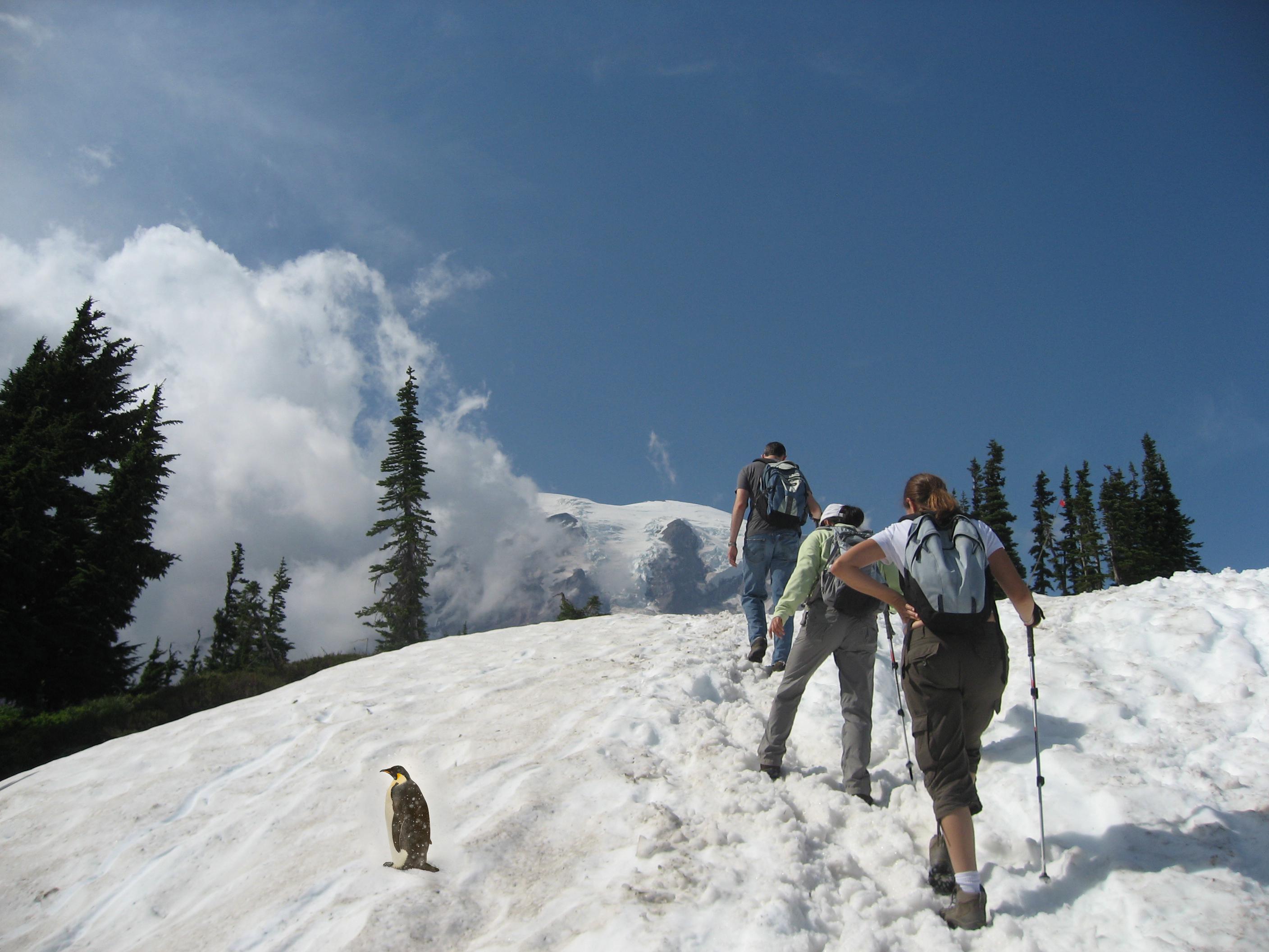
"Hikers Encounter Surprise Penguin"
Source
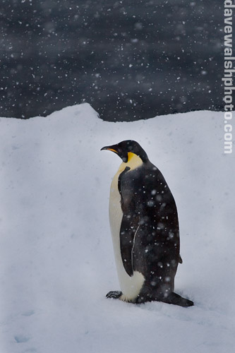
Target
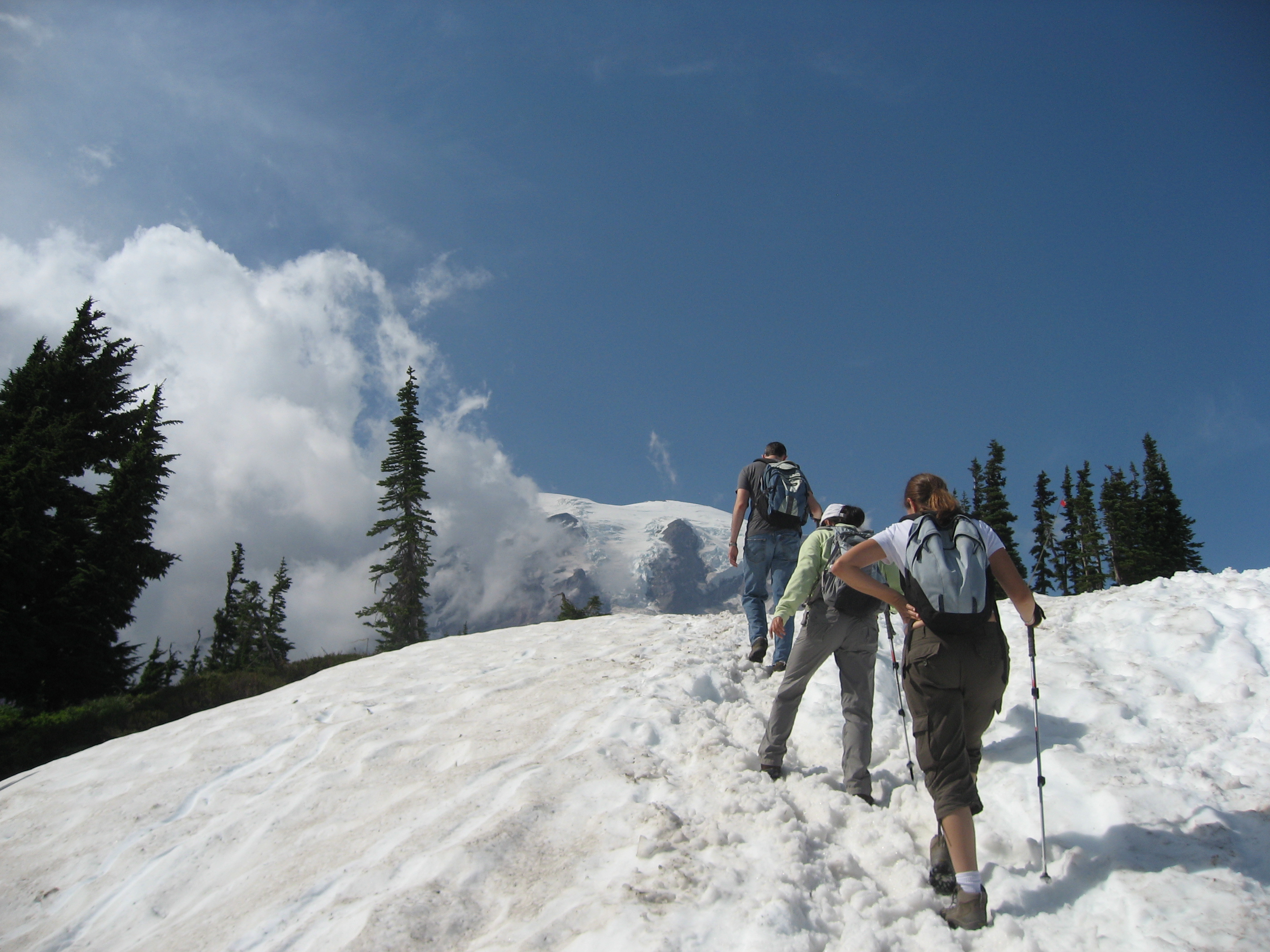
Source Copied onto Target
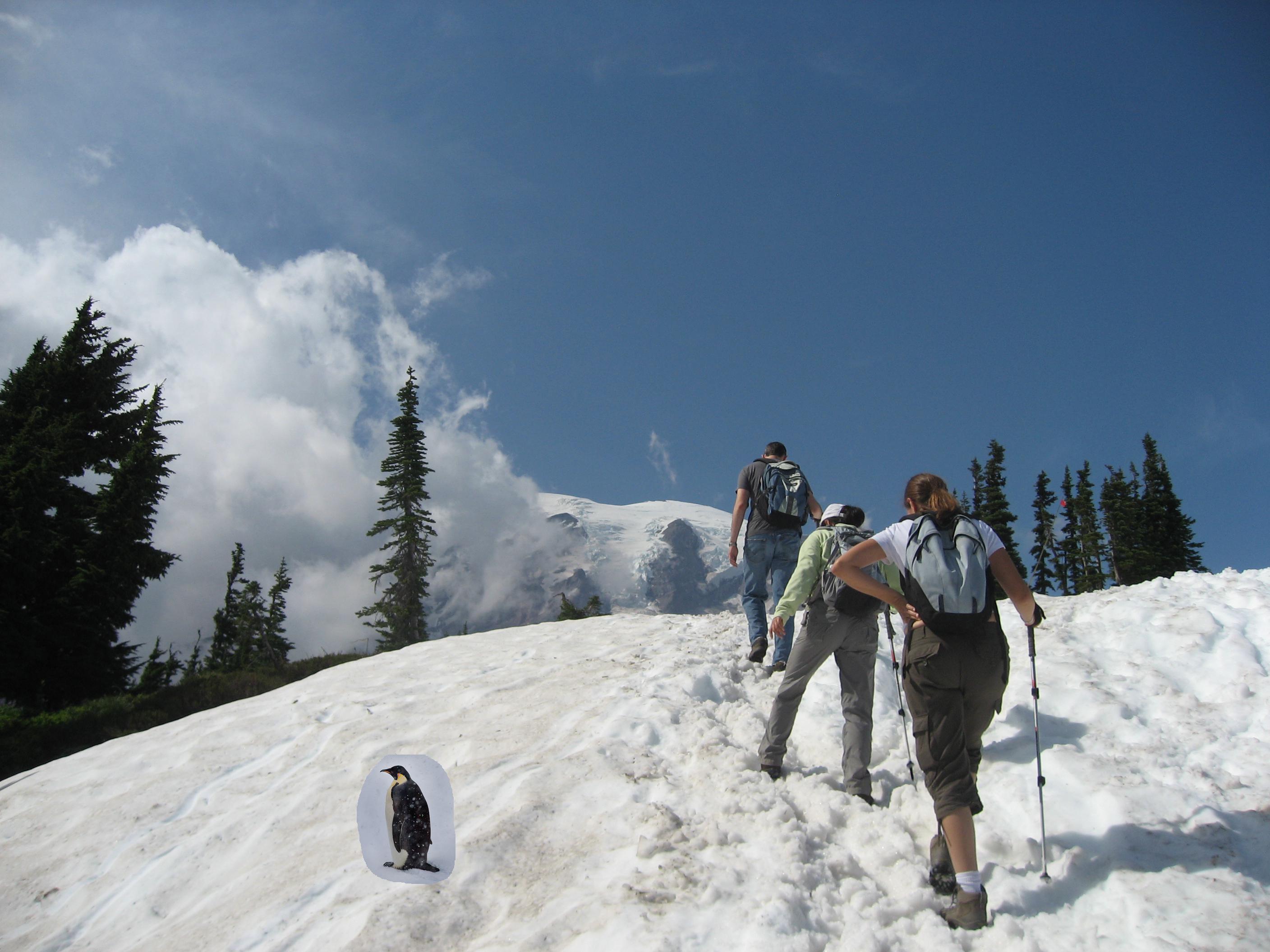
Blended Result
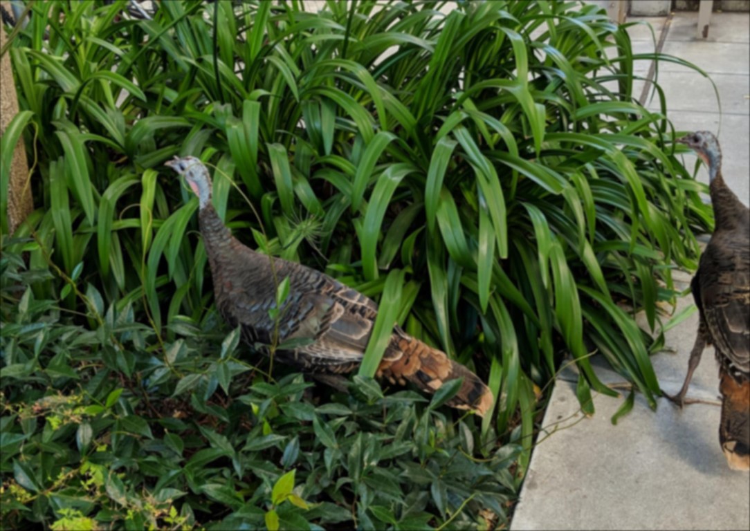
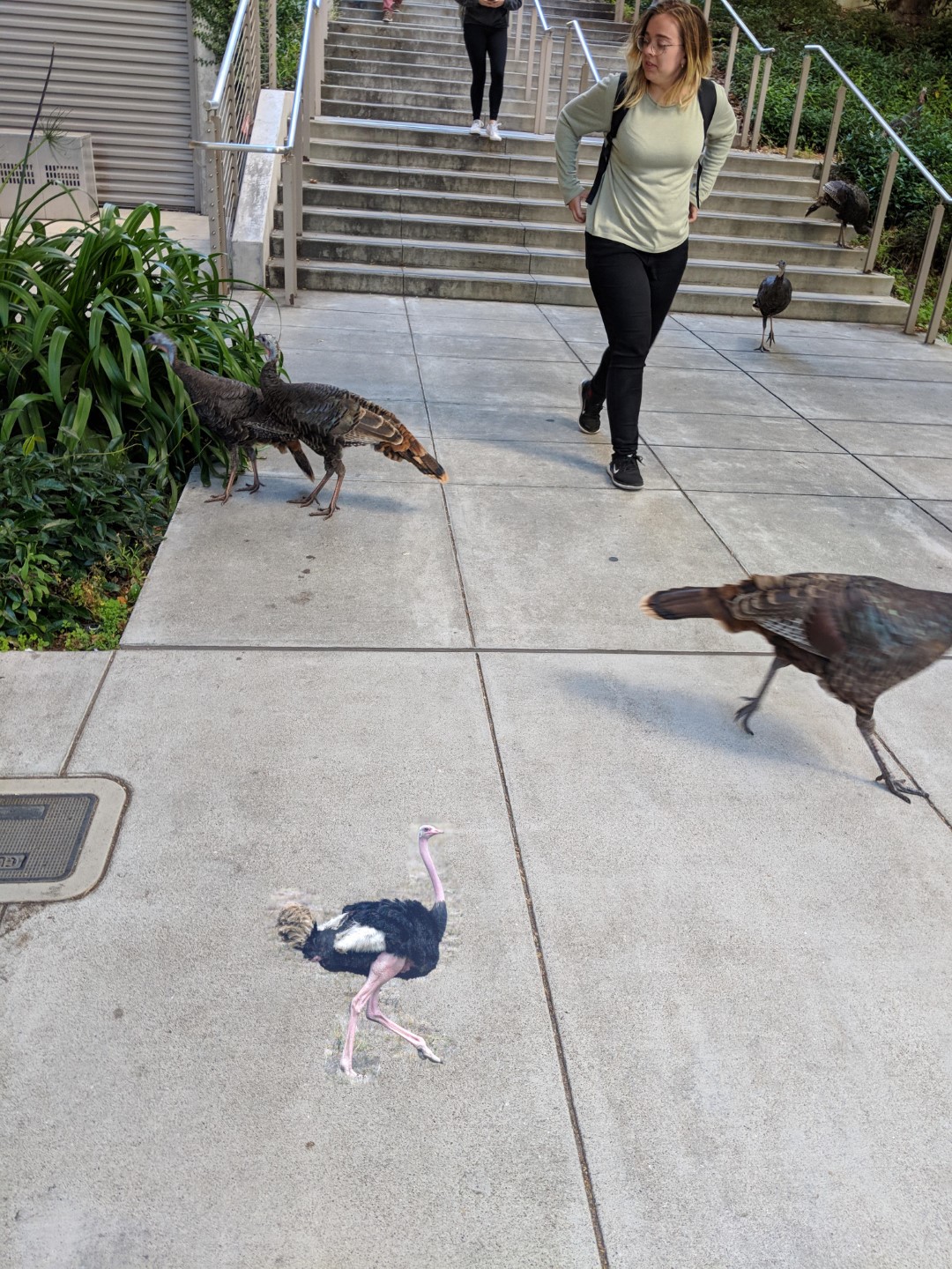
"Since We Have Turkeys On Campus, Why Not Bigger Turkeys (Ostriches) Too?"
Source
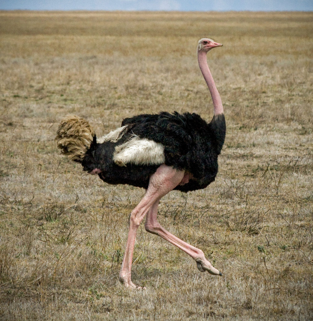
Target
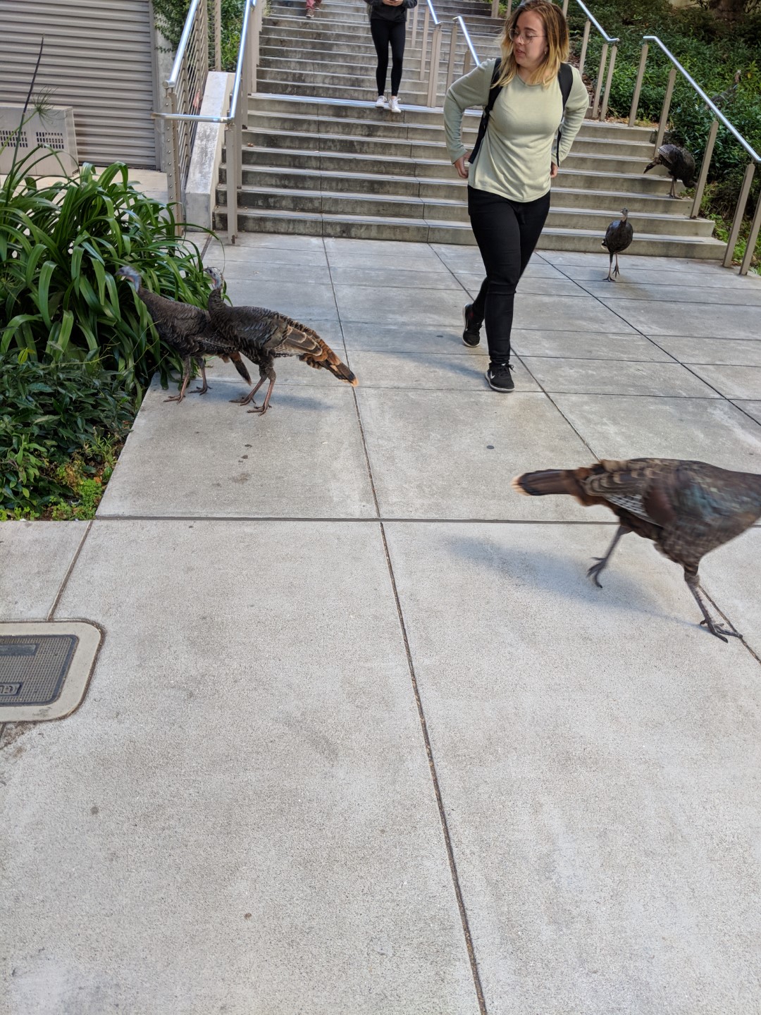
Source Copied onto Target
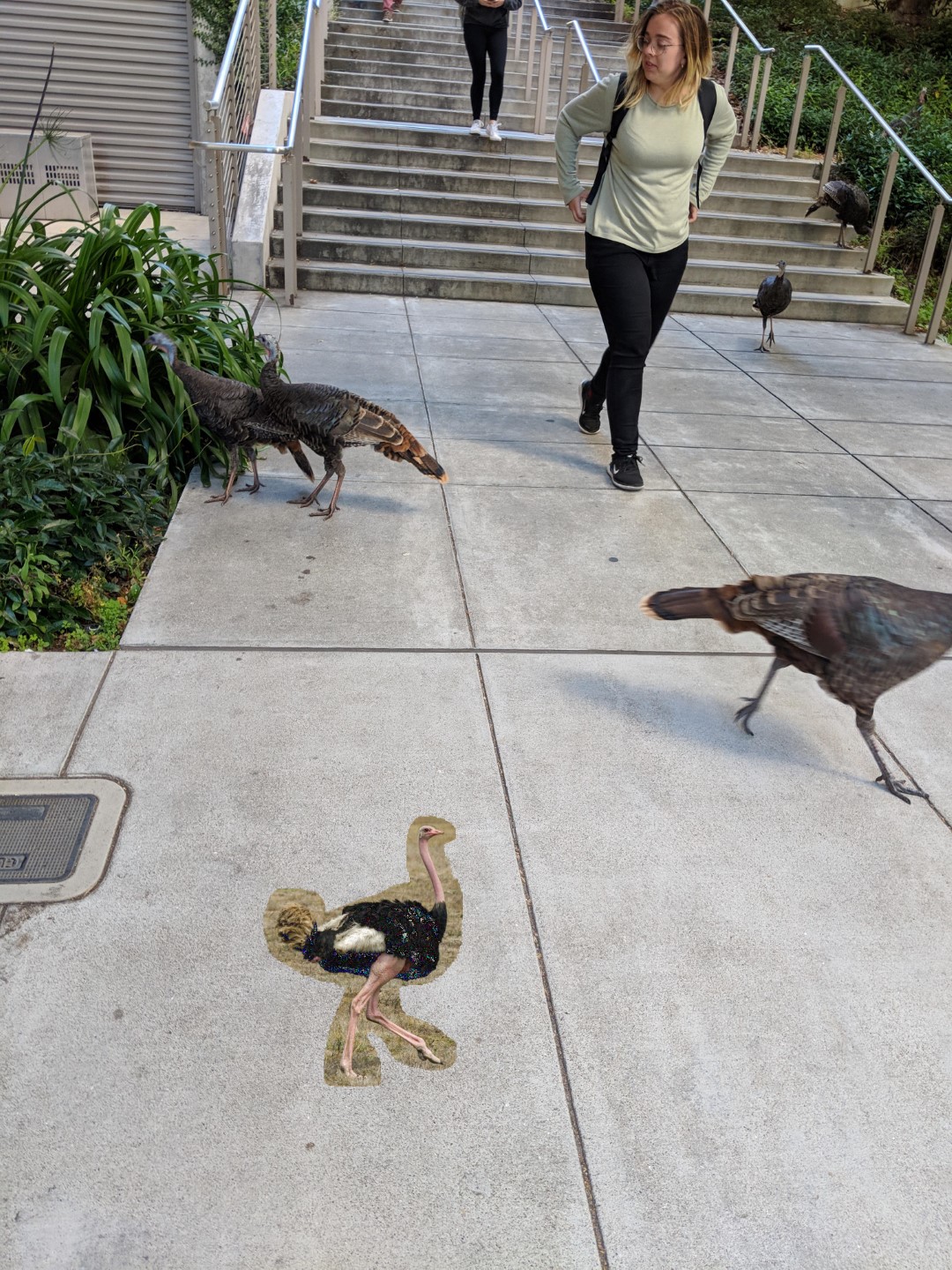
Blended Result
"EECS Tattoo"
Source
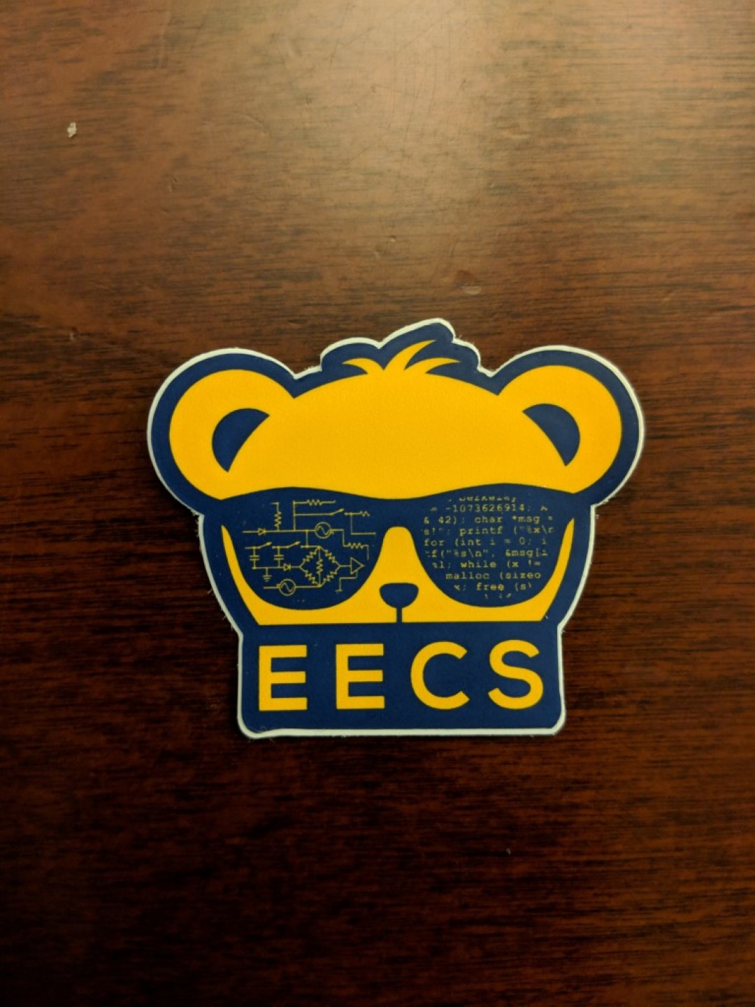
Target
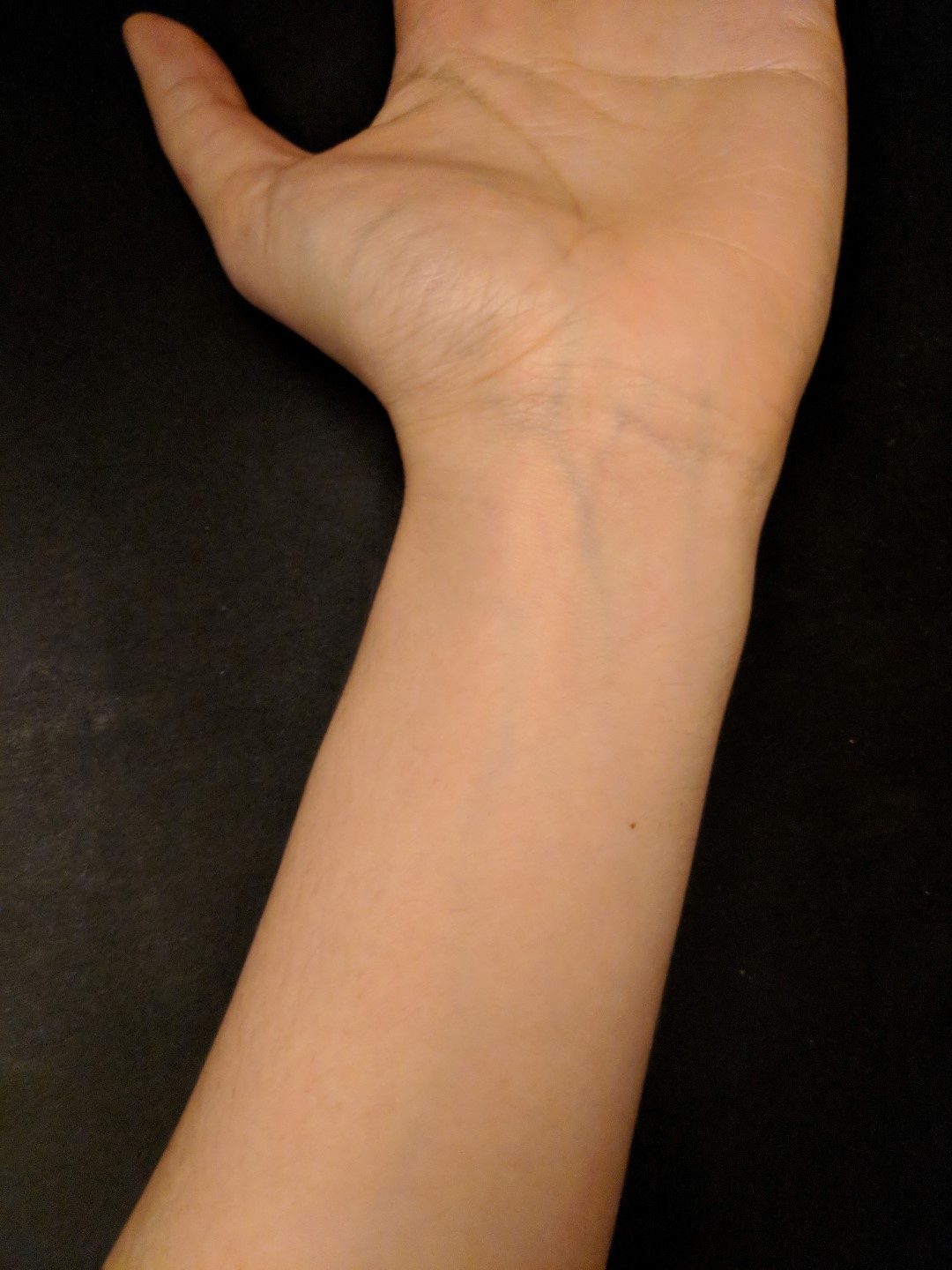
Source Copied onto Target
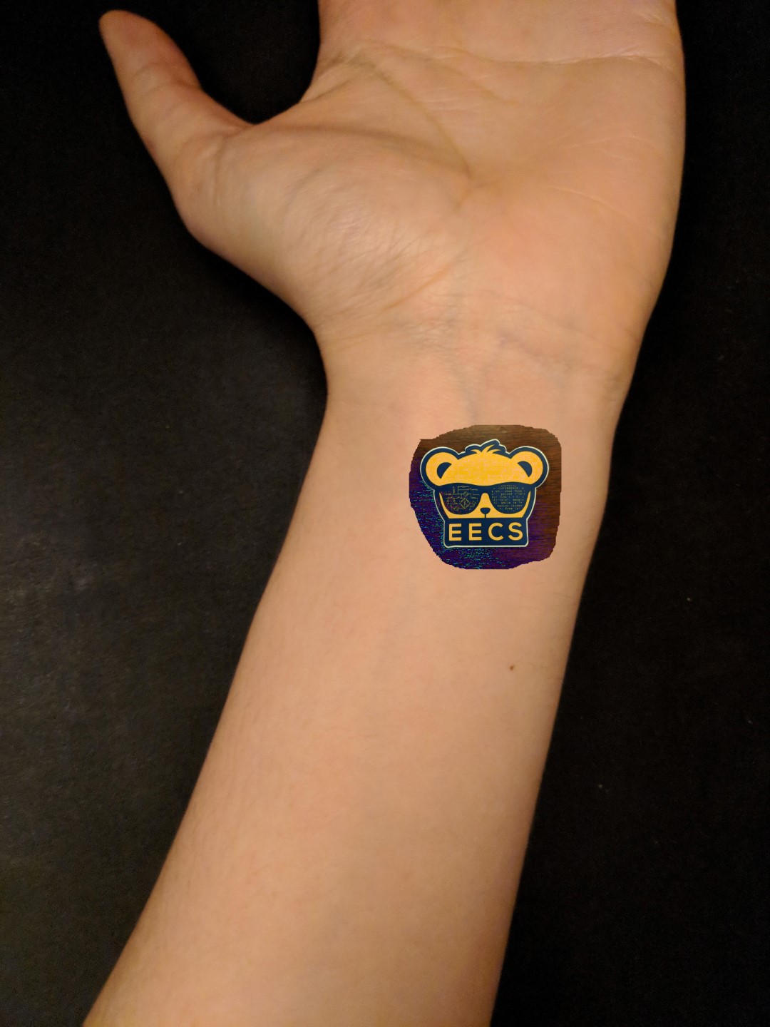
Blended Result
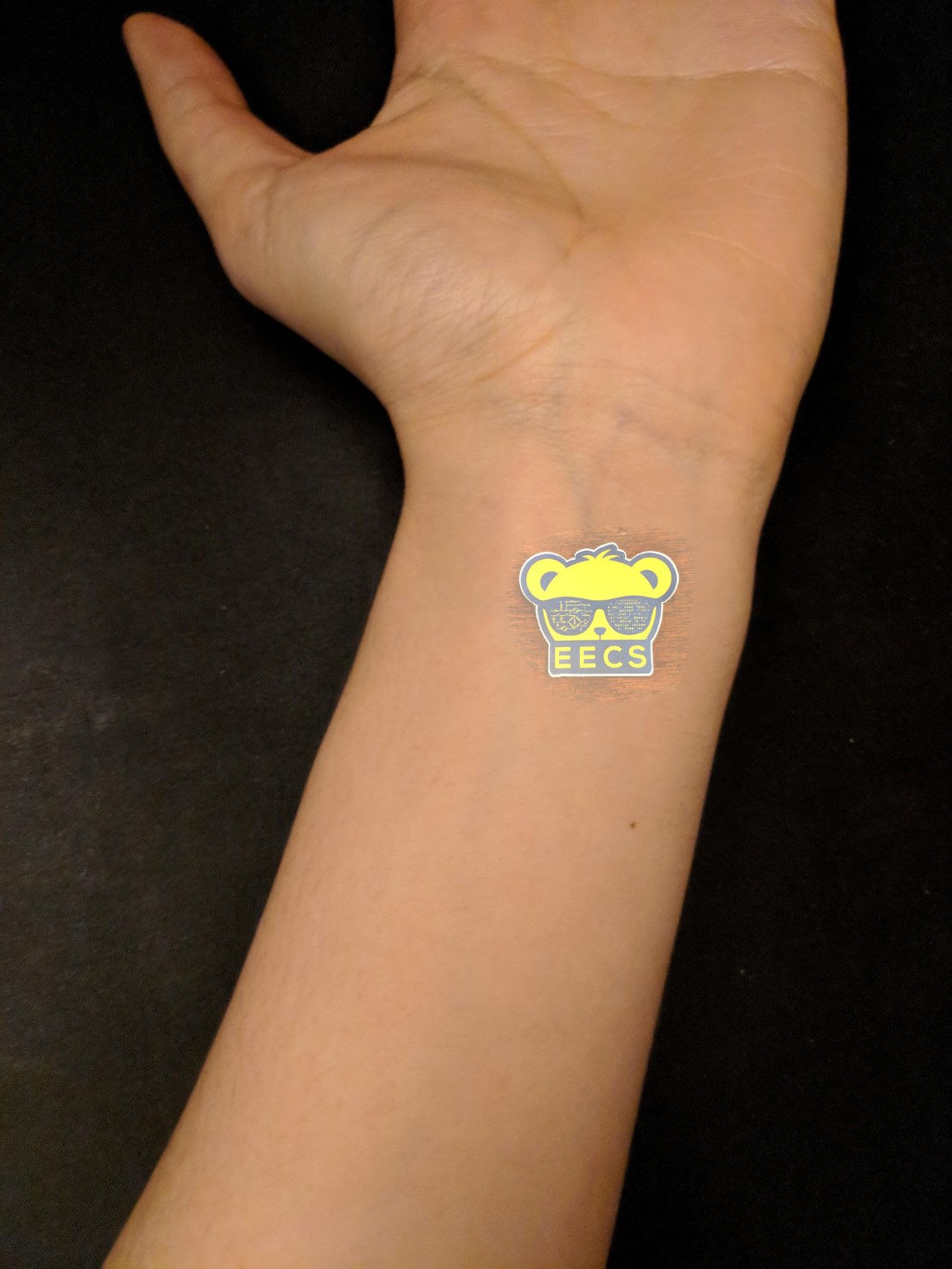
It's pretty arguable that the last blended image ("EECS Tattoo") is a "failure" in that the colors and white balance seem so off, especially from the original. It just seems like an unnatural brightness for everything else surrounding it. (You might say the same for the "Ostrich" image as well, though that image also seems off for perspective reasons and because ostriches are much bigger in real life.)
This results because our algorithm only cares about relative gradients. Thus, it won't necessarily hold any colors inside the source image constant, changing any colors as necessary so that the boundary gradients match for the target image. Nevertheless, it is still a step up from directly copying the source onto the target.
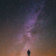
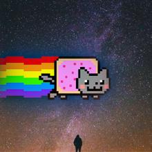
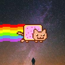
Now let's return to one of the images we produced for Part 1.4 - "Space Cat!"
With multiresolution blending, it looked like this:
With Poisson blending, it looks like this:
It could probably be argued that neither results are 100% perfect, and thus there are pros and cons to either approach. The multiresolution blending is less computationally intensive than solving a massive least-squares problem, for one. For another, the original colors of the source image are much better preserved. However, there is a blue "halo" around the source image because this form of blending doesn't attempt to match gradients between the source and target images to make the colors of the boundary feel completely seamless or fitting.
Meanwhile, the Poisson blending does a much better job of matching the colors surrounding the source image, maintaining a lot of the color gradients of the milky way background. On the other hand, it can only do this by greatly modifying the colors of the internal pixels to keep the internal gradients relatively constant. As a result, our cat is colored very differently - in a way, these colors agree with the mood of the rest of the target image a bit more, but they also aren't very faithful to our original source if those colors are what we want to keep.
In other words, a trade-off exists between these two forms of blending. On the one hand, multiresolution blending can give you faithful source colors inside the mask while sacrificing color-consistency with the target image at the mask's boundaries. On the other hand, Poisson blending can give you color-consistency at the mask's boundaries while sacrificing faithfulness to source image colors inside the mask.
Conclusions
Perhaps the most important thing I have learned from this project is the idea that we can perform very powerful image manipulations by leaving the domain of pixels - thinking in other domains unlocks new models in which very complicated problems become a little simpler and more elegant. For example, Poisson blending is pretty powerful, doing what would be very difficult to compute just based on pixels and instead taking advantage of the underlying structure in images that's there in their gradients.
Beyond that, by comparing multiresolution and Poisson blending, I can appreciate that different image manipulation techniques all have their pros and cons. Sometimes certain techniques are cheaper but less effective, and sometimes there is no "right" technique - you just use the one suitable for your use case(s) depending on the trade-offs you're willing to make.
Citations
To produce Gaussian kernels throughout this project, I used the source code from this StackOverflow post.
All Part 2.2 masks EXCEPT the Nyan Cat mask were created using Python script written by Tianrui Guo, linked in this Piazza post. The Nyan Cat mask is the same as in Part 1.4, and it was produced in Photoshop.