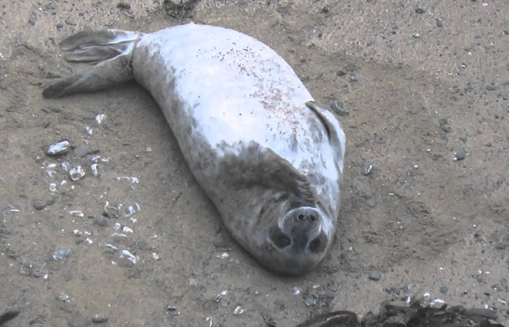
Figure 1: Normal Seal

Figure 2: Sharpened Seal
Part1.1: Image Sharpening
The picture of the seal was sharpened by applying a averaging kernel of 3x3 with each element being 1/9. cv2.filter2D applied the kernel to the image and the resulting smooth image was subtracted out to sharpen it. The two images can be seen below.
Figure 1: Normal Seal
Figure 2: Sharpened Seal
Part1.2: Hybrid Images
I followed the instructions and I created a gaussian kernel for each picture. Then I make the low frequency of both images using scipy.signal.convolve2d and then for the high frequency one I created the high frequency by subtracting the original from the low frequency. At the end I combine the high and the low and return it.
One of the issues I ran into was determining the size of the kernel. I mainly just used trial and error but on average the larger the picture the larger the kernel.
As for colour I noticed that using colour generally enhances the effect especially with the Bear-Tiger hybrid. Below is the black and white for each one as well as the colour.
Also below is an example of a failure. This one resulted because the kernel size was not appropriate and the two images have very different contrasts and thus resulted in just one image showing as the other one was blurred to oblivion.
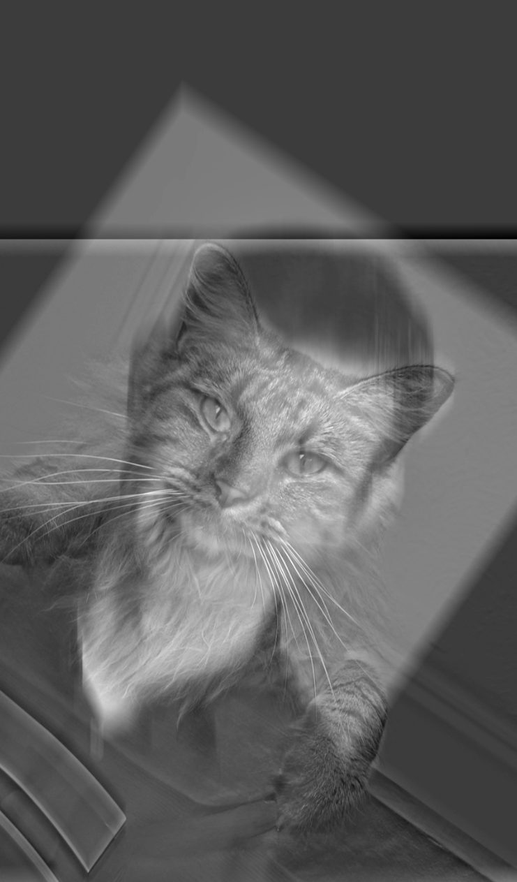
Figure 1: BW derek nutmeg
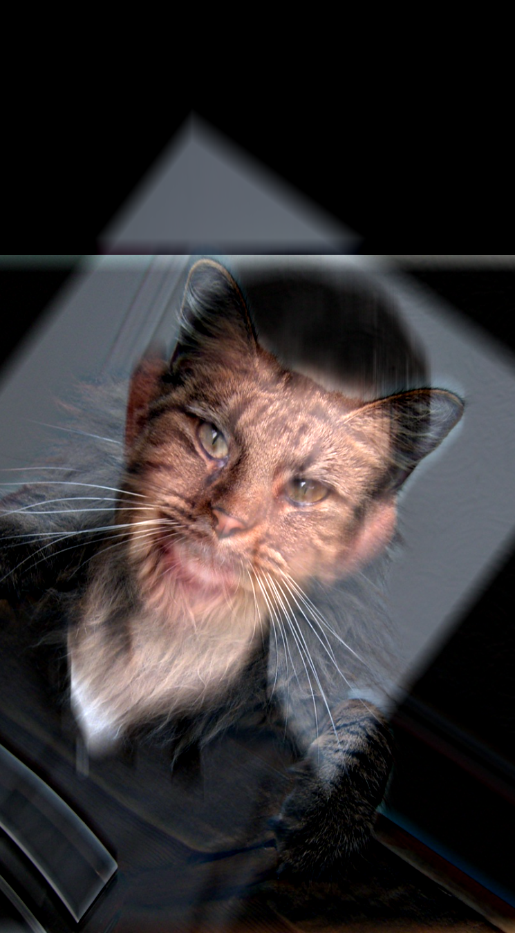
Figure 2: Colour derek nutmeg
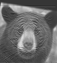
Figure 3: BW bear tiger
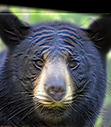
Figure 4: Colour bear tiger
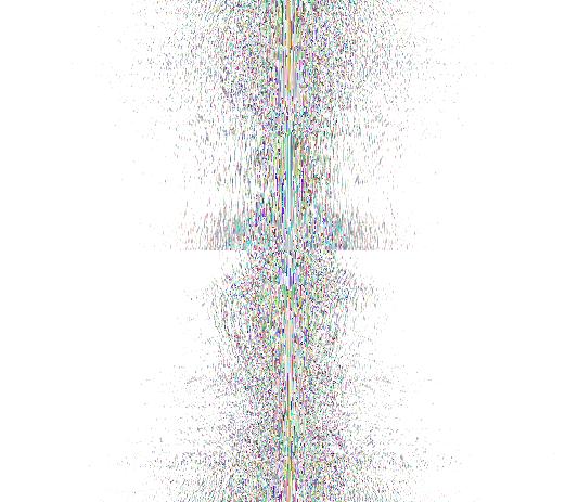
Figure 5: Bear frequency
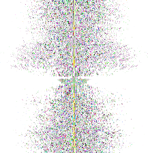
Figure 6: Tiger frequency
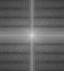
Figure 7: Bear filter frequency
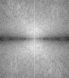
Figure 8: Tiger filter frequency
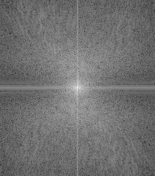
Figure 9: Combined frequency
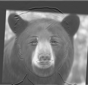
Figure 8: BW bear jack
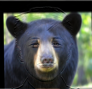
Figure 9: Colour bear jack
Figure 10: a failure example. Other image blurred to oblivion due to too high of a kernel size.
Part1.3: Gaussian and Laplacian stacks
The gaussian were made simply by first creating a gaussian kernel and then repeatedly applying it on the original image. One issue I ran into was the fact that cv2.getGaussianKernel returns a 1d kernel so I had to multiply it with it's own transpose to make it 2d.
The lapacian stack was made by subtracting the latest gaussian iteration from the last one seen.
The last element of the laplacian stack was made the same as the last item of the gaussian stack.
Part1.4: Multiresolution Blending
First I make a mask by making one half of the image black and the other half white. Then I apply the process described by the paper to construct the blended imaged from my respective gaussian and lapacian stacks.

Figure 1: the apple

Figure 2: the orange
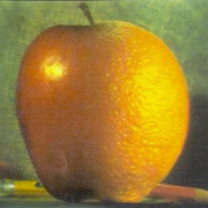
Figure 3: the applange
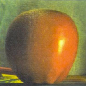
Figure 4: the oraple
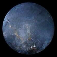
Figure 1: the frypan bottom
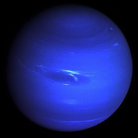
Figure 2: the neptune
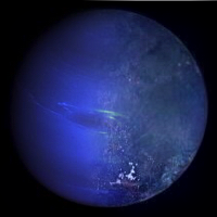
Figure 3: the fry pan neptune fusion
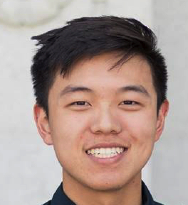
Figure 1: the jack
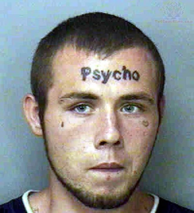
Figure 2: the psycho
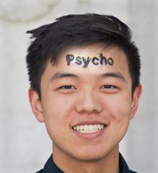
Figure 3: the psycho jack.
Overview of part 2
For part two, most of the challenge is applying the same concepts of the toy problem (which was rather trivial with the objective functions given) to the harder objective function of the poisson merging. But once it was implemented it worked rather beautifully in achieving the desired results.
Part2.1: Toy Problem
For this part I simply populated the A matrix with the objective function as given and then solved it with least squares to get back the original image.
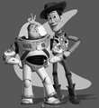
Figure 1: the reconstructed image
Part2.2: Poisson Blending
The first step of this problem was the figure out the objective function like in the toy problem. After some scratch work done on paper, I figured out the objective function which is rather similar to the toy problem. Then i got to work implementing the problem. The key is to understand the minimization equation. Essentially what it is saying is to find an image such that the difference at the borders is minimized and also the difference between neighbors in the new image is maintained as the original. So basically what it does is that it shifts the entire colouring of the source image to match it at the borders.
To implement it, I used the starter code linked on piazza to generate the masks. Once I had the masks, I wrote a function to match the source to the destination and create a naive paste-in result (v in the equation); it also returned offsets so I can index back into the source image for border information for the border cases.
Once that was done, it was only a matter of running the objective function with the masks as info to populate the A matrix and b vector and solve it like any other least squares problem. A few problems I ran into was first, I used a normal np array as my A matrix and it soon made my 8 gigabytes of memory dissappear. This was ameilorated by using a lil.matrix (my new rapper name) to populate it and then turn into a csr matrix to do the least squares. This significantly sped up the process. Also I ran into some values being too high so a simple clip at the very end solved that.
Other than that most of the pictures turned out pretty well, at least in terms of colour. However, if the background of the images do not match then there is no hope (look at the bear in woods example). The one failure I had was when I tried pasting a battleship in a tea cup. The resulting image turned the battleship gold. This is because in the source image the colouration of the battleship was very close to that of the water it sat in so when it got put in the tea cup, the water turned gold to match the target image and the battleship turned gold with it.
Lastly I compared the difference between poisson blending vs the multiresolution blending. Read more about it at the bottom.
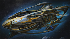
Figure 1: the source image
Figure 2: the source mask

Figure 3: the target image
Figure 4: the target mask
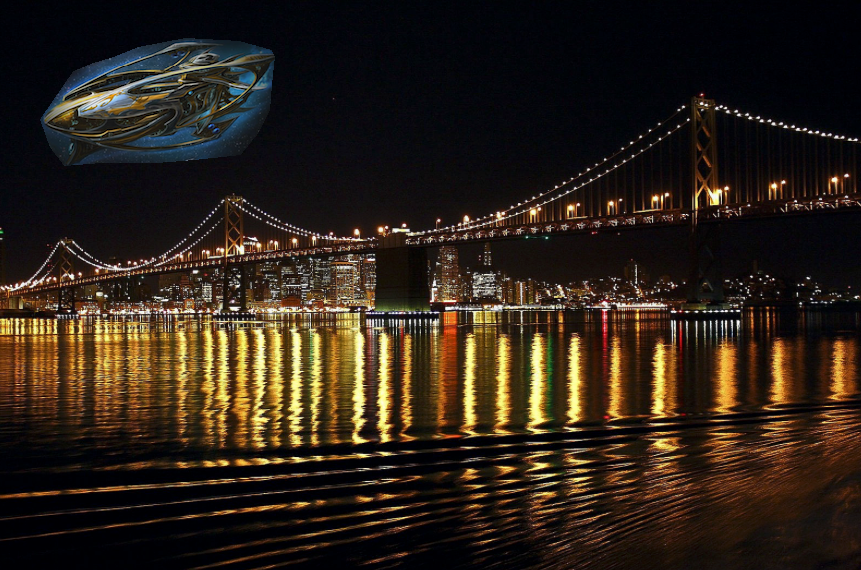
Figure 5: the naive result
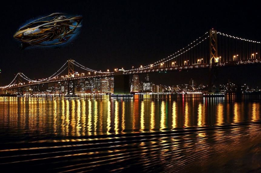
Figure 6: the blended result

Figure 5: the naive result
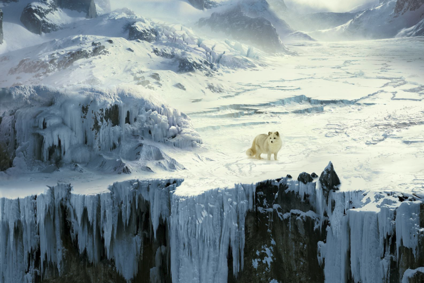
Figure 6: the blended result
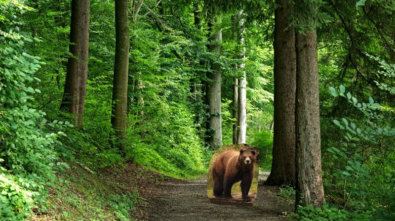
Figure 5: the naive result
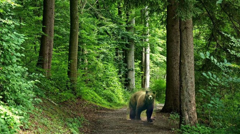
Figure 6: the blended result. While the colours still look right, it doesn't look natural because the background's objects differ
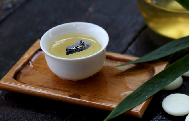
Figure 5: the naive result
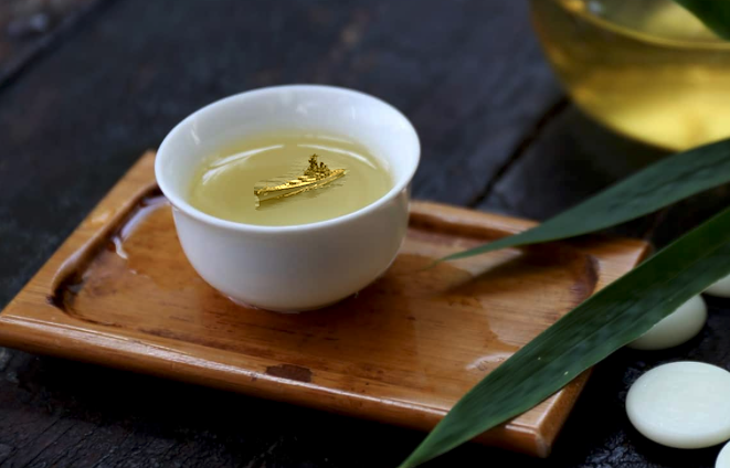
Figure 6: the blended result. The battleship turns gold because it was too similar to the original water which got turned gold to match the tea.
Figure 1: the jack
Figure 2: the psycho
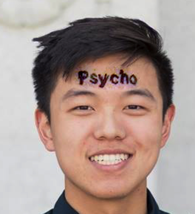
Figure 3: using poisson blending
Figure 4: using stacks blending