Overview

For this assignment/project, we worked with frequency domain and gradient domains to try to "photoshop" images, mainly interweave one part of a source image to another so that it looks natural.

Part 1: Frequency Domain

1.1 Warm-up

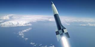
For the first part, we worked in frequency domain. We saw that to sharpen an image, one should take the high filtered part of an image, which is the original image - low filtered image, multiply it by a constant, and add it back to the original image. Here is an example of it working!

1.2 Hybrid Images

To create the hybrid images, we notice that when we are close, we observe high frequency components better and when we are further, we notice the low frequency components better. So, if we have two images A,B and we want to create a hybrid image that shows A more clearly when close and B more clearly when far, we take the high filtered image of A and low filtered image of B and add them together!

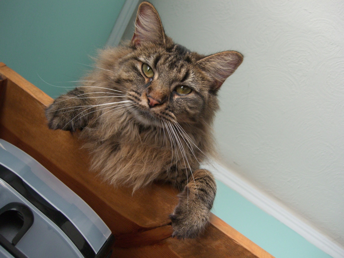
Here are some picturesque images! Apologies for the spacing of Derek and Nutmeg... I can't get them to go close for some odd reason.

Favorite Picture is Derek and Nutmeg

Owl and Cat (FAILURE CASE)

SHREK and PEPE (GOOD CASE)

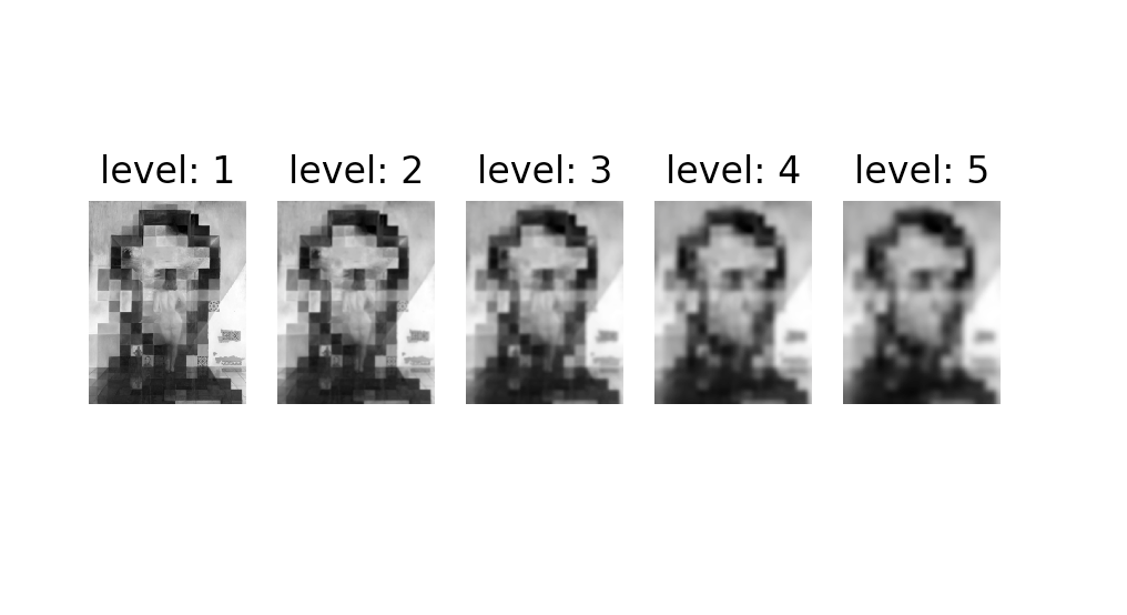
1.3 LAPLACIAN AND GAUSSIAN

HERE IS AN EXAMPLE WITH LINCOLN

1.4 Multiresolution Blending

This was interesting. If we want to "blend" two images together, a naive approach would be to just take the part you want from image A and put it onto image B. However, this is terrible in that there are obvious seams and discrepancies that anyone could tell from looking at the combination. Instead, multiresolution blending uses laplacian and gaussian stacks to achieve a smooth blend.

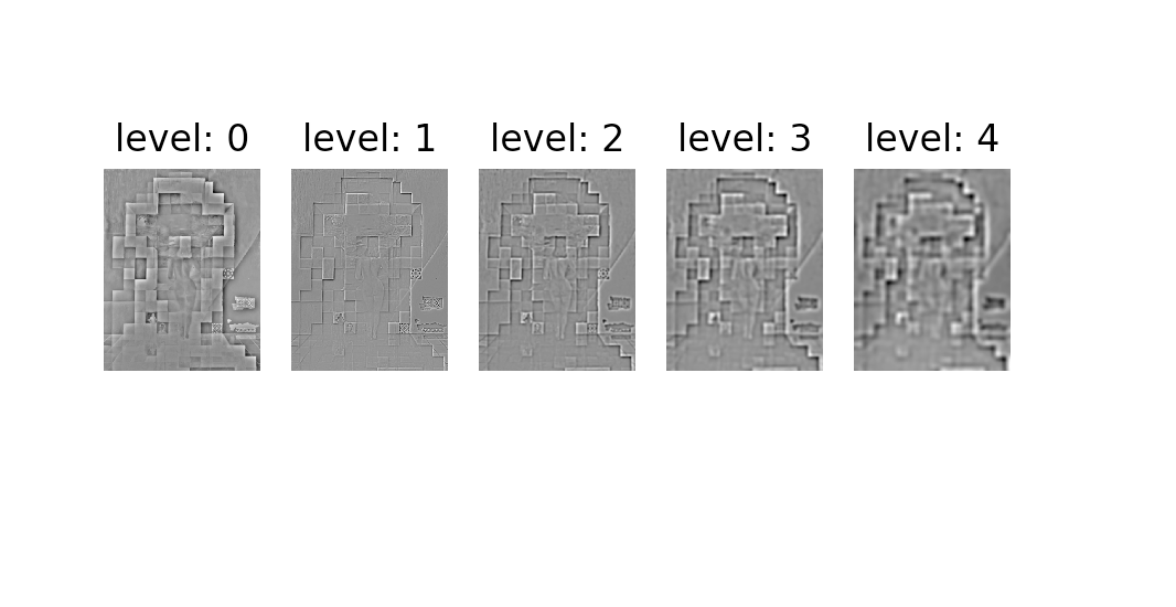
What we need is a mask to select which part of image A we would need. We get the gaussian stack of the mask, the laplacian stack of A, and the Laplacian stack of B. The Laplacian stack is calculated via first getting the gaussian stack G[0, 1, .. n-1]. Then, L[i] = G[i] - G[i+1] for i = 1, ..., n-2, and L[0] = I - G[0] and the last layer is same as the gaussian stack's so that L[0] + L[1] + ... + L[n] = I - G[0] + (G[0] - G[1]) + ... (G[n-2] - G[n-1])+ G[n-1] = I!!

After getting the laplacian stacks of the two images (L1, L2) and gaussian stack of the mask (G1), the new image's laplacian stack (L3) is the follows: L3[i] = L1[i] * G1[i] + L2[i] * (1 - G1[i]), where G[i] sort of acts like weights for the laplacian stacks. Then, we get the final blended image by summing up the levels in L3 to produce the image!

For the images below, the first row is the orange laplacian weighted by the 1 - mask gaussian. The second row is the apple laplacian weighted by the mask gaussian.

Here's a cool one with a bottle on the sea.

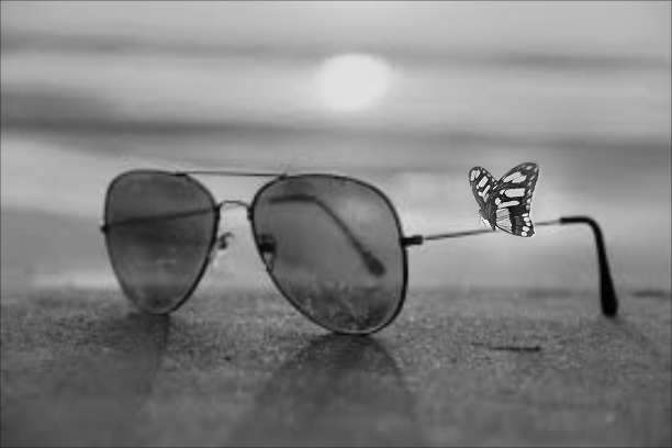
Here's a nice one with a butterfly and sunglasses.

Part 2: Gradient Domain Fusion

This part of the project focused on gradient-domain processing, more specifically "Poisson Blending". This is just looking at the x,y gradients of the source image and taking them into account when pasting it onto the target image. We want the final picture to conserve the gradients of the source picture part while adjust to the pixel intensities of the target image. This involves many enforcements on each pixel, as we want the difference of the final pixel and its neighbors to be the exact same as the difference in the source pixel and its neighbors.

We try this simply with the toy problem. We simply enforce x,y gradients of the final image to be the same as the original (there is no source here), and we also enforce that the left corner pixel of the final image is the same intensity (rgb values) as the original. Basically this (copied and pasted from problem task):

we do this for each and every pixel. For me, I made a one pixel border and did it for the pixels inside the border since it's a pain to do boundary conditions, and it turned out fine. We plug into the scipy.sparse.linalg.lsqr solver, and it does fine!

1.	minimize ( v(x+1,y)-v(x,y) - (s(x+1,y)-s(x,y)) )^2	the x-gradients of v should closely match the x-gradients of s
2.	minimize ( v(x,y+1)-v(x,y) - (s(x,y+1)-s(x,y)) )^2	the y-gradients of v should closely match the y-gradients of s
3.	minimize (v(1,1)-s(1,1))^2	The top left corners of the two images should be the same color

Part 2.1: Toy Problem

For the first part, I began by working with a small example to illustrate gradient domain processing and correctly figure out the math involved. I achieved this by computing the x and y gradients from an image s and then using all the gradients, plus one pixel intensity, to reconstruct an image v. Here are the original and reconstructed images side by side:

Part 2.2: Poisson Blending

This was my favorite picture to blend! OBSERVE CAREFULLY. Here is what I did: I extended the above toy problem to now take into account four neighbors instead of two (so the x gradient constraint doubles since you enforce p, p-1 and p, p+1 and same as y gradient). Then, there is a new problem: What happens if the pixel p is on the mask boundary (aka for example, the pixel to the right of p is outside the mask)? We answer that by imposing a constraint for those types of pixels. Instead of enforcing their x,y gradients to match the source, we make the difference between p of the final image and the target image's p neighbor (neighbor of the same position) gradients match. Here is what I mean:

Where N represents the four neighbors of i (up, down, left, right). For a neighbor that is not in the mask, we draw from the target image and use that pixel instead.

FAVORITE

HERE ARE SOME OTHER ONES

If you look at the one above, it kinda failed in that the background didn't completely blend in well with the man. This is because the background colors were wayy too different, which leads to just overall confusing in coloring of the pixels. Also, it may be because one is a painting and other is a photograph

Here is the bottle again with POISSON BLENDING. Let's take a look.

Here's a cool one with a bottle on the sea.

Personally, I think the poisson method worked better since it even emulated the sea's boundary with the bottle and also encapsulated the bottle's glass and made it see through to the trees beyond. Anyways, it was cool!