Part 1: Frequency Domain
Part 1.1: Warmup
In order to sharpen a select image, I created an unsharpening mask by constructing a Gaussian kernel with a sigma = 3. In theory, an image is sharpened if a high-pass filter is passed onto the original image. This high-pass filter can be made by subtracting the original image by the image with the Gaussian filter.
 Original Image |
 Sharpened Image |
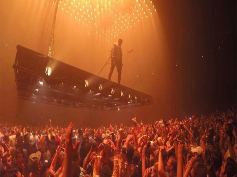
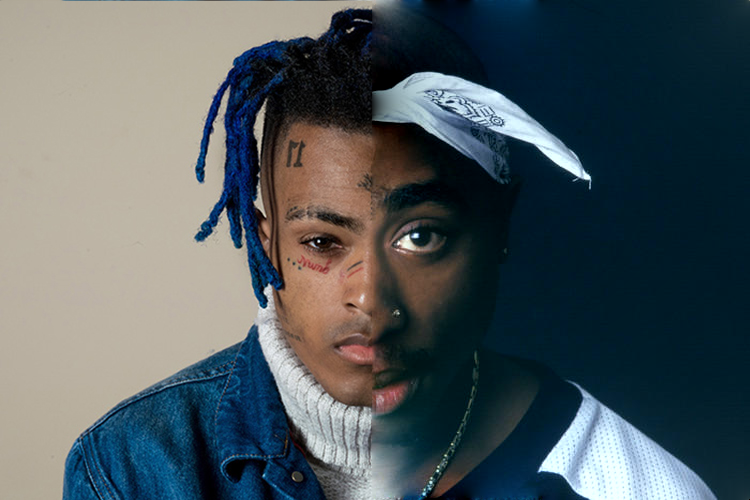
Part 1.2: Hybrid Images
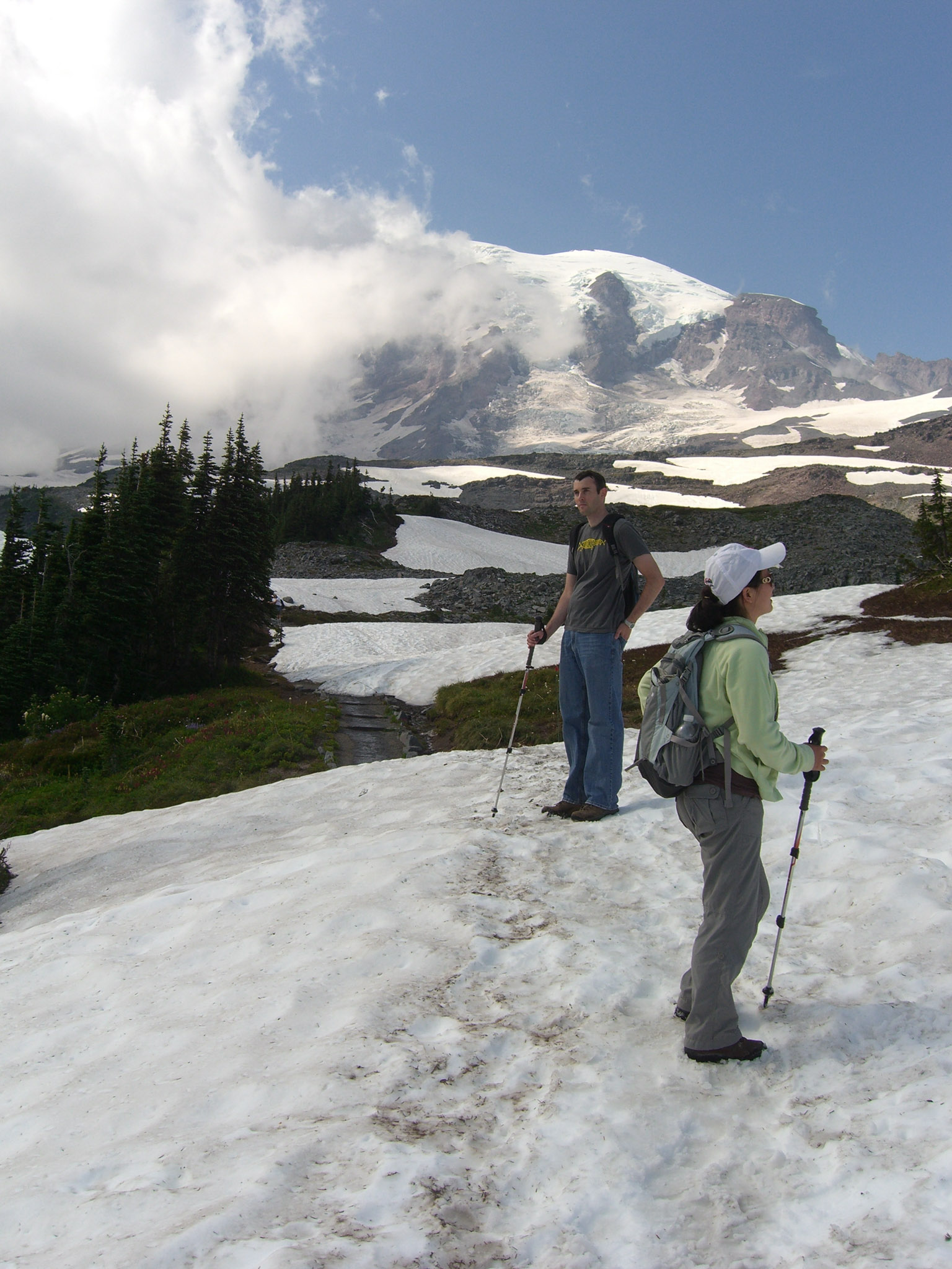
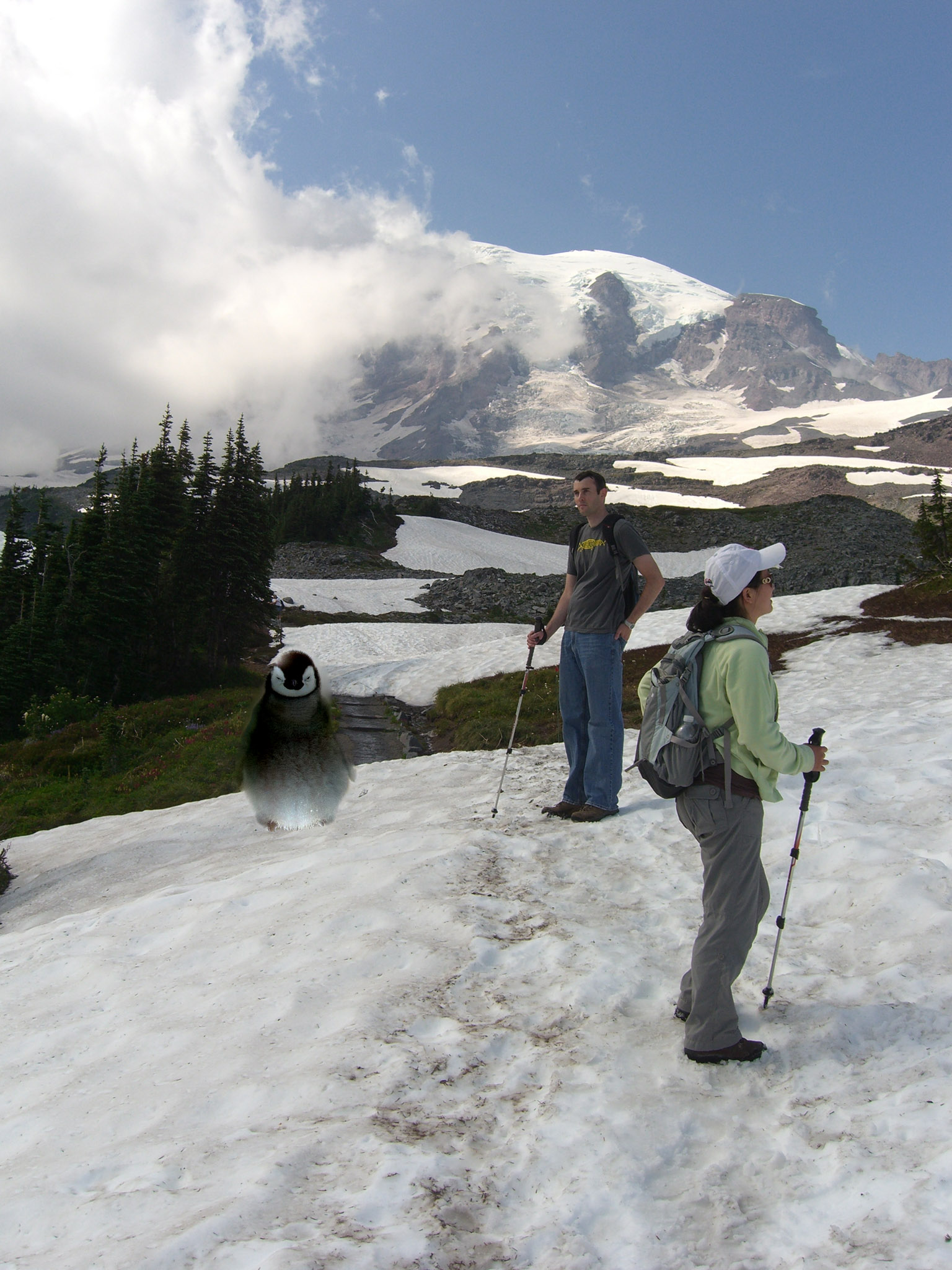
A hybrid image can be constructed by combining an image with a low-pass filter and an image with a high-pass filter. This results in an image where one can view only the low frequences from a distance, and one can view the high frequences when looking at the image closely. For the following successful images, the low-pass images have a sigma value of 3 and the high-pass images have a sigma value of 5.
|
|

|
||

|

|

|

|

|
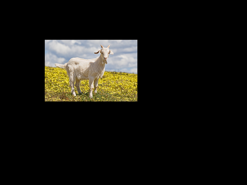
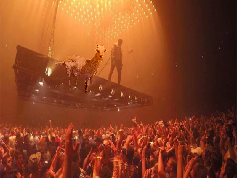
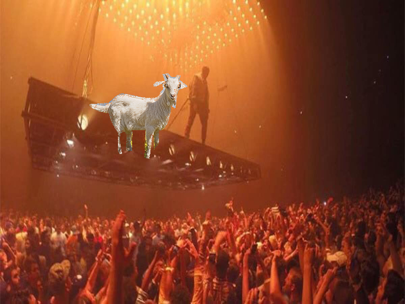
Here are two more examples: one success and one failure. The goat in the kanye-goat hybrid does not showup instantly; one has to squint very closely to see a mere outline of the goat.

Kanye West and a goat, failure. |

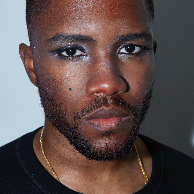
MC Ride from Death Grips and JPEGMAFIA. |
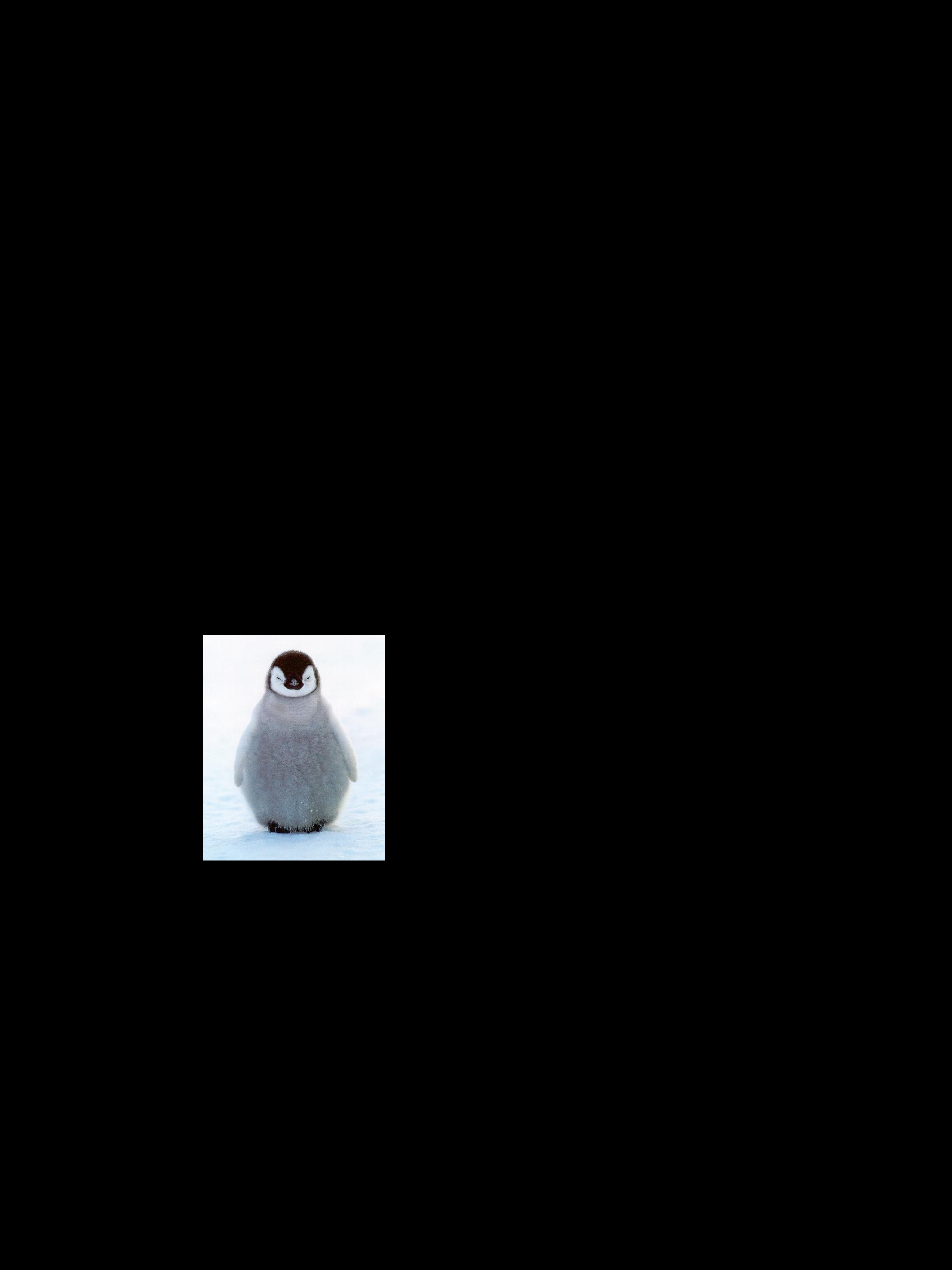
Part 1.3: Gaussian and Laplacian Stacks
I created gaussian and laplacian stacks to analyze a particular image's structure. The stacks were made such that a filter was repeatedly applied to an image with a sigma of 2. The laplacian stacks were the differences between a previous gaussian filter and a stronger gaussian filter. The last level of the laplacian stack, however, is the same as the gaussian stack in order to superimpose the image.

|

|

|

|

|

|

|

|

|

|
Part 1.4: Multiresolution Blending
To create a multiresolutional blend, we want to perform the following algorithm:
Build laplacian pyramids for both images A and B, and a gaussian pyramid for the region mask. Then form a combined pyramid such that for each level, we compute the following equation: GR(i, j) * LA(i, j) + (1 - GR(i, j)) * LB(i, j). Lastly, we construct a blended image by flattening all of the combined stacks into one image.

|

|

|

|

|

|

|

|

|

|

|

|
Part 2: Gradient Domain Fusion
Part 2.1: Toy Problem
For the toy problem, we construct an image using the horizontal and vertical gradients. I constructed a sparse matrix A of dimensions 2*height*width + 1 and height*width. I minimized the x and y gradients of the target image to match the original image. I also made sure that the top left corners of both images were exactly the same.

|
|
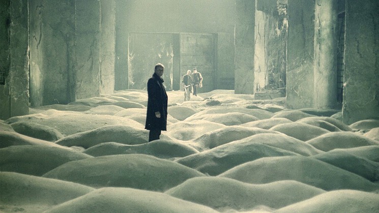
Part 2.2: Poisson Blending
Instead of looking at the gradients, I looked at the center pixel's neighbors. Thus, my sparse matrix consists of (4 * x * y, height * width), for x and y are the dimensions of the array im2var. Note that if the pixels aren't inside the mask, then I simply set the result pixel's intensity to the target pixel's intensity.
|
|
|
|
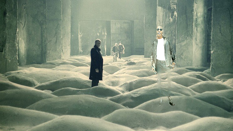
There is an obvious difference between simply copy and pasting the source mask to the target image, and using poisson blending; the seams between the two images are very obvious.
|
|
|
|
|
|
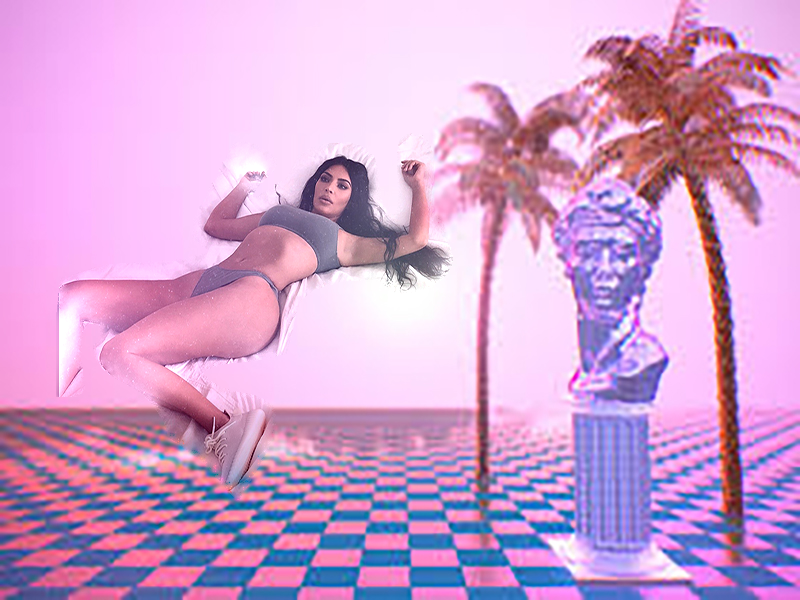
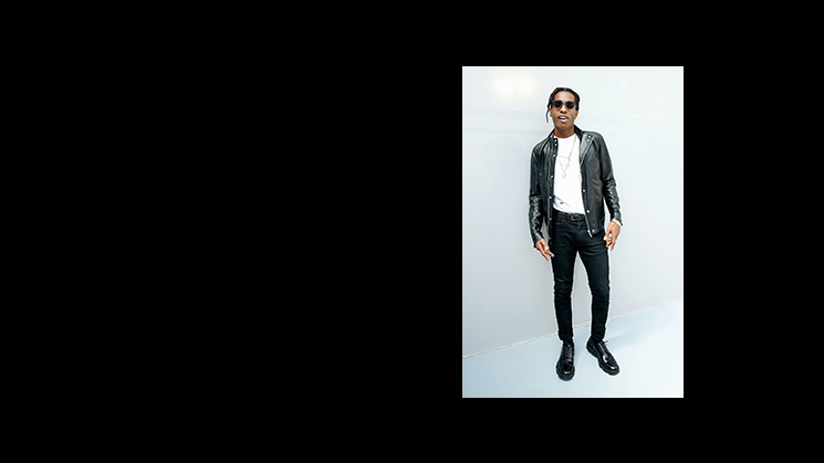
The blend below failed due to how different the backgrounds were. A$AP Rocky's pants blend in with the background, which is not intended at all.
|
|
|
Laplacian Pyramid vs Poisson Blending
Though the blended photo on the left is grayscale, there exists some differences between the laplacian pyramid and poisson blending. When it comes to multiresolutional blending, only the edges are blended. On the other hand, poisson blending seeks to preserve the color intensities during the blending, making the blend less obvious.

|

|

|
|