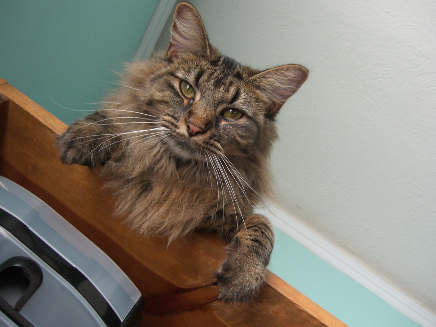
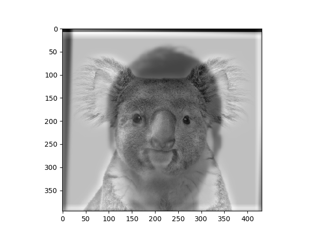
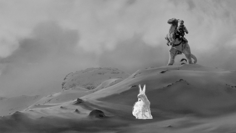
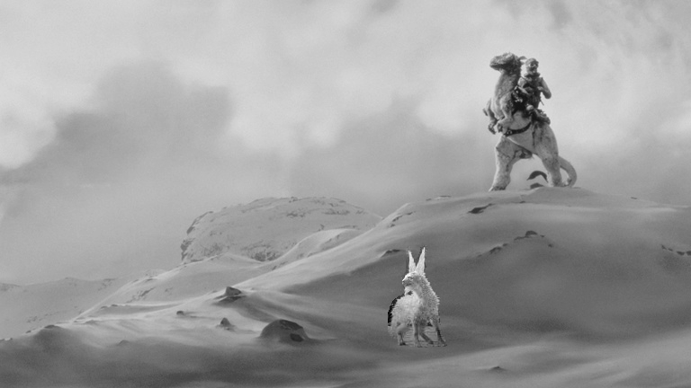
The first thing we tried to get familiar with image processing for this project was to "sharpen" an image using a gaussian filter. The basic idea is that we can apply a gaussian filter to an image and then subtract the result from the original image to identify edges in the image. By adding the edges back to the original picture we obtain an image that is "sharper" than the original image. This process is shown in the three pictures below.
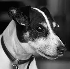
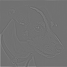
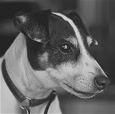
We can see that the dog's collar gets a little bit sharper, in addition to flecks of white on the dog's neck being more visible. The overall image gets slightly darker so the sharpening is somewhat hard to see.
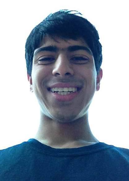
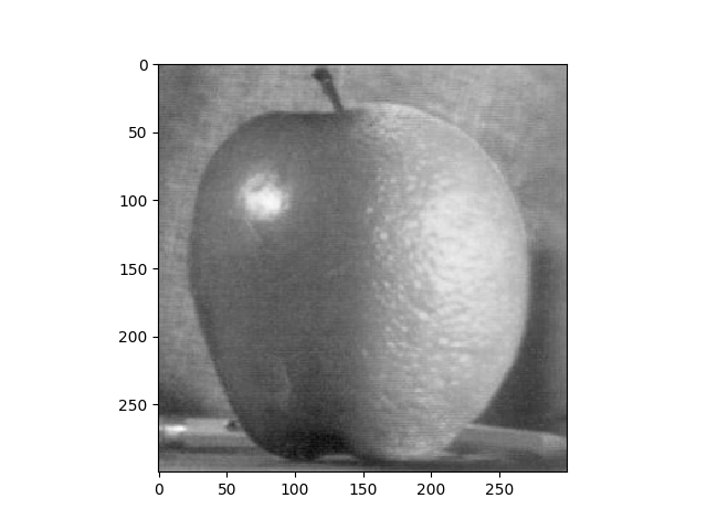
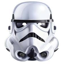
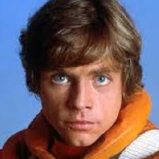
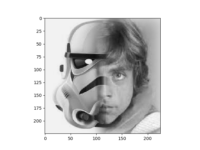
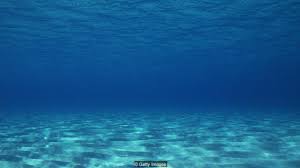
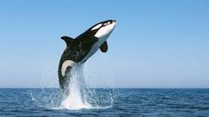
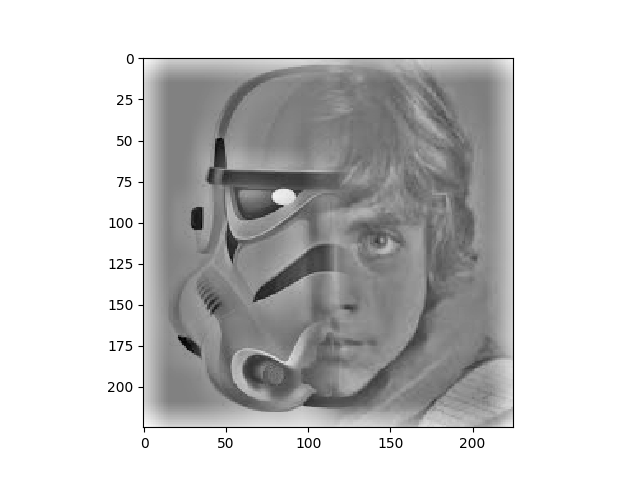
In hybrid images we are aiming to make images that are perceived differently at different distances. To accomplish this we start with two images and apply a low-pass filter to one and a high-pass filter to another. By aligning and combining the two images filtered in this way we can create an image that looks like one thing close up (where you perceive the high frequencies) and another when viewed from far away (when the low frequencies dominate). Examples of hybrid images and their source pictures are below.
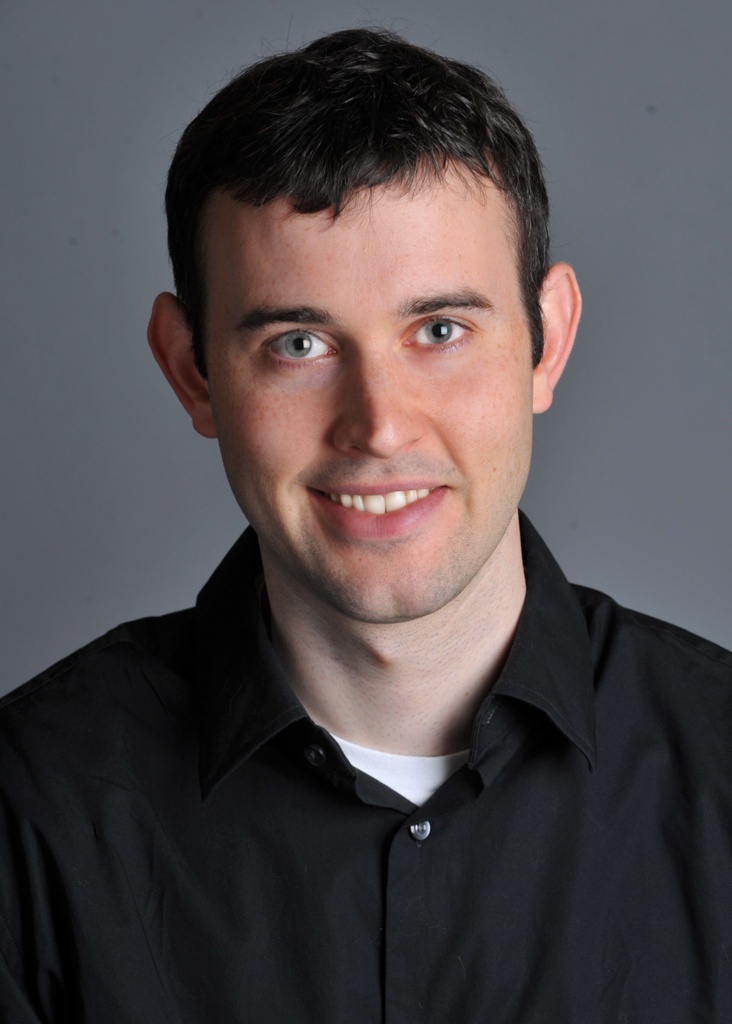
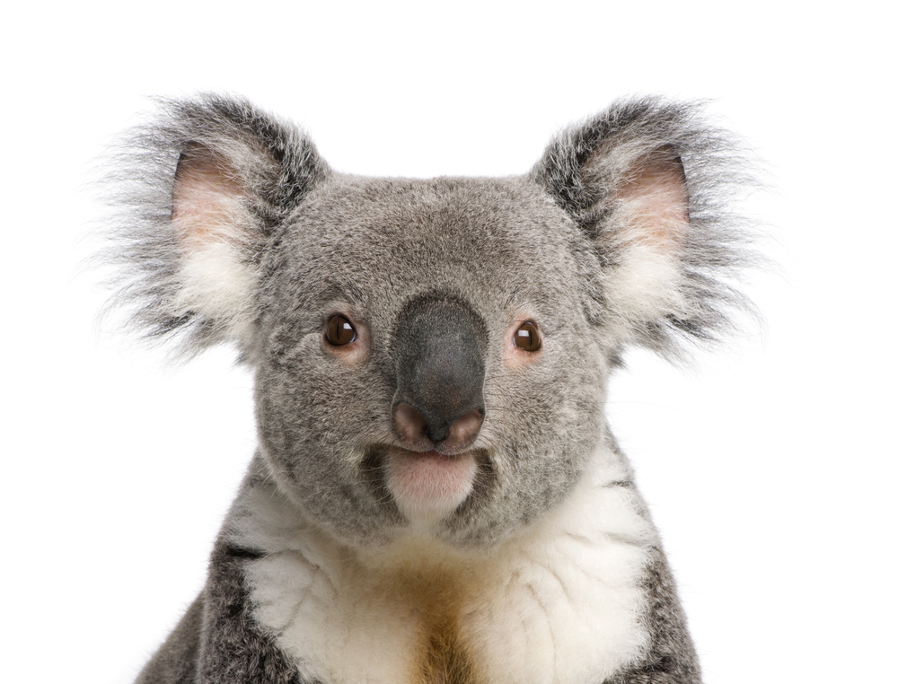
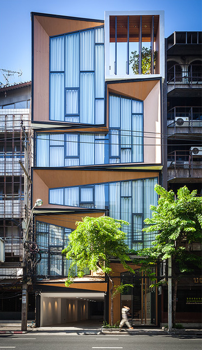
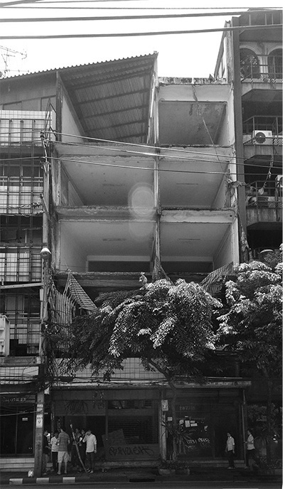
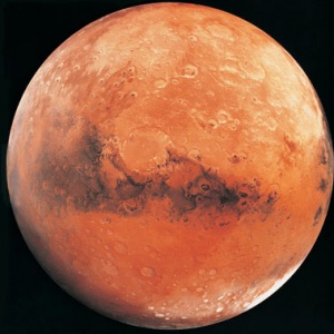
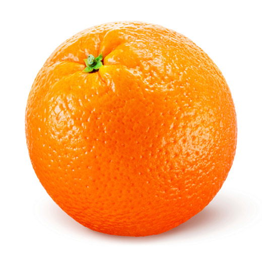
We can see that in these examples the technique seems to work better on faces than on the objects. The blending of Mars and the orange is probably not succesful because the images are too similar and so it is difficult to draw a big distinction between the two images apart from texture, which blends together when the images are combined.
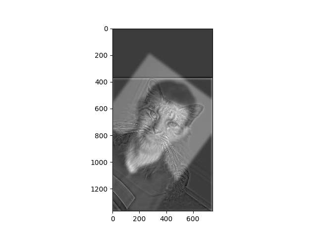
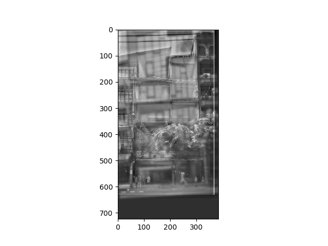
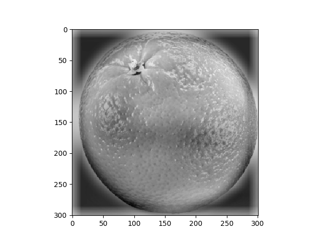
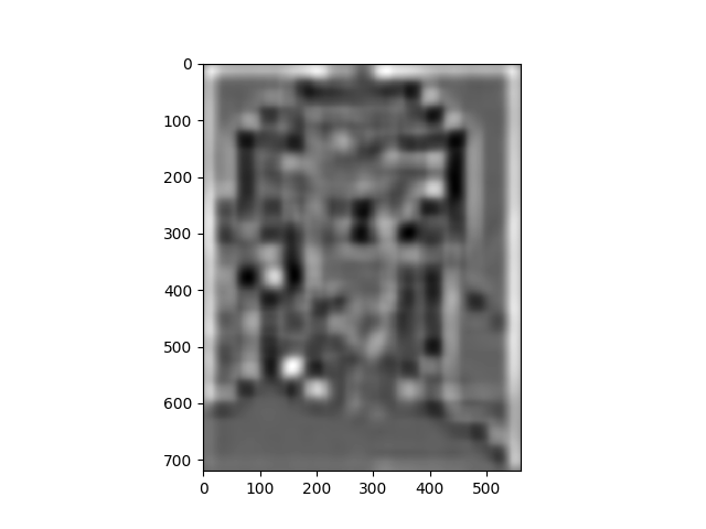
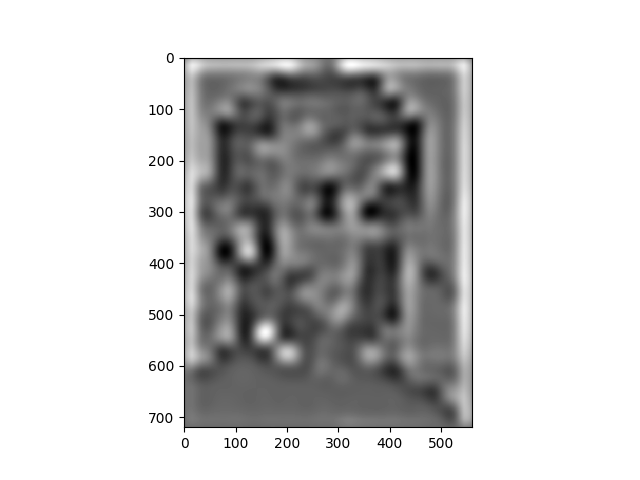
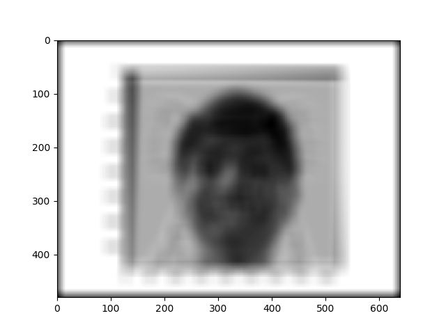
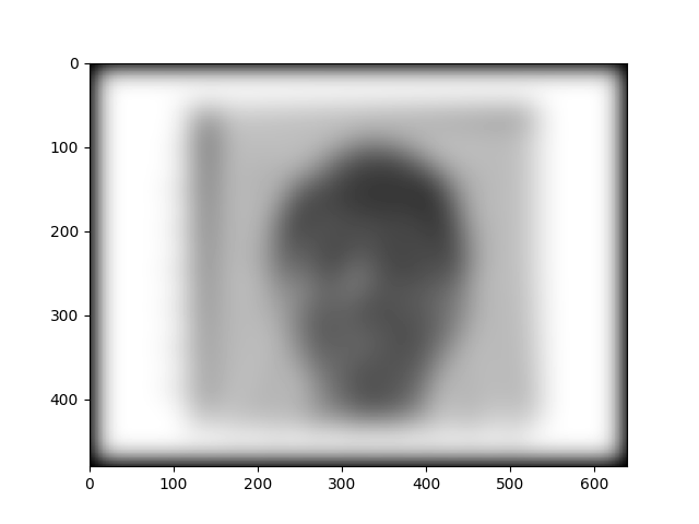
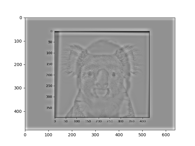
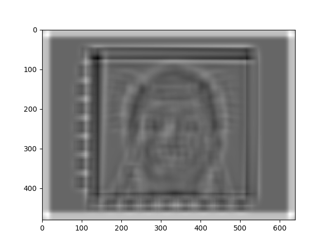
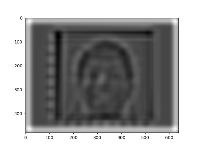
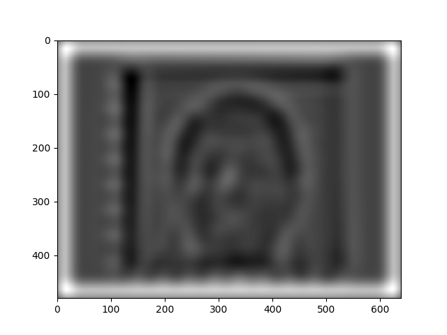
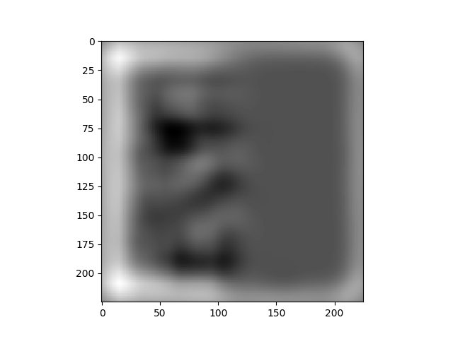
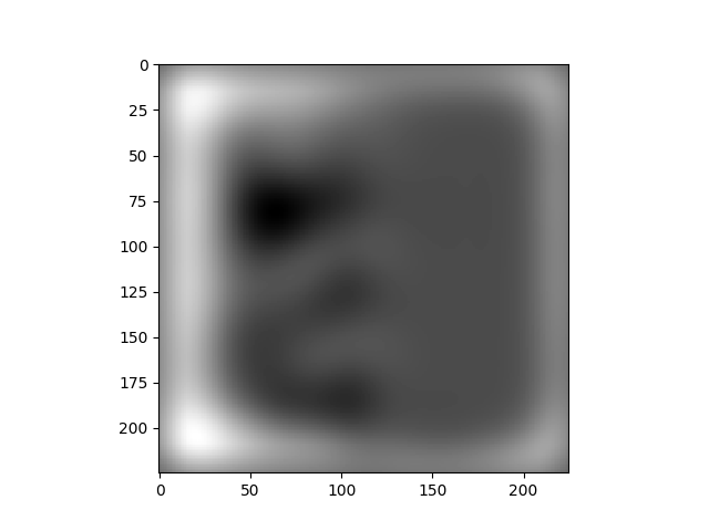
To further illustrate the process we can look at the log magnitude of the images to see which frequences are being filtered away. Included below (in order) are the log magnitude of the two original images for the koala example, the two filtered images, and the final image.

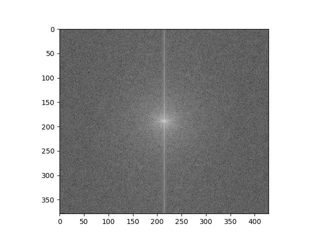
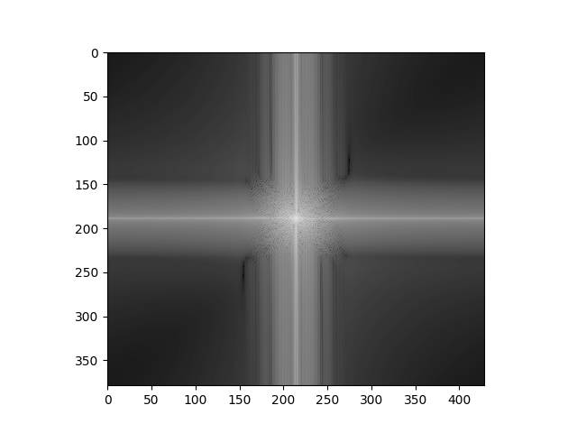
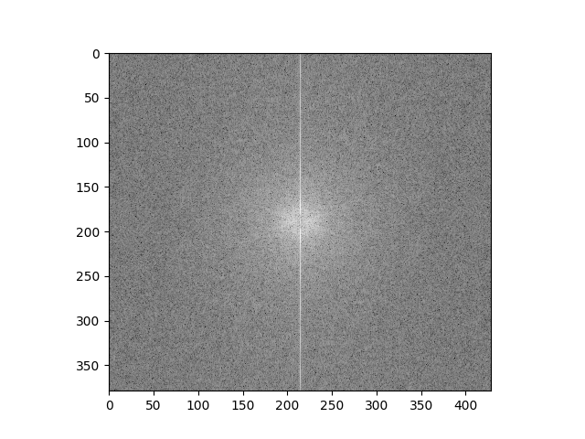

We can especially see the filtering in the 3rd image, where the high frequences are removed.
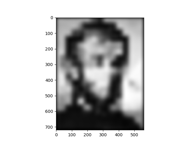
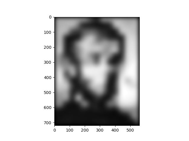
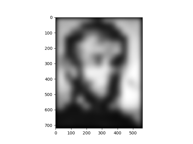
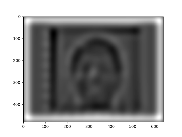
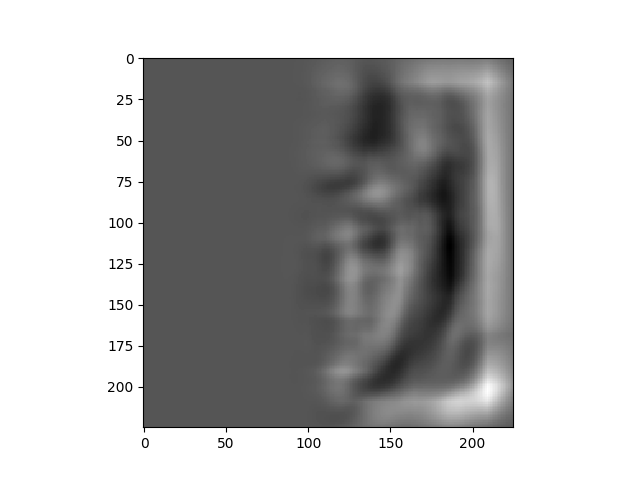
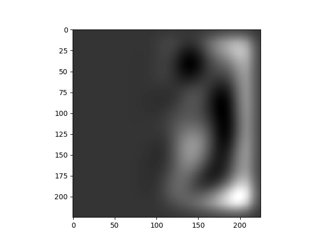
Gaussian and Laplacian stacks enable us to analyze images by revealing what an image looks like at different frequency bands. Below we both of these stacks applied to the picture of Lincoln By Salvador Dali.
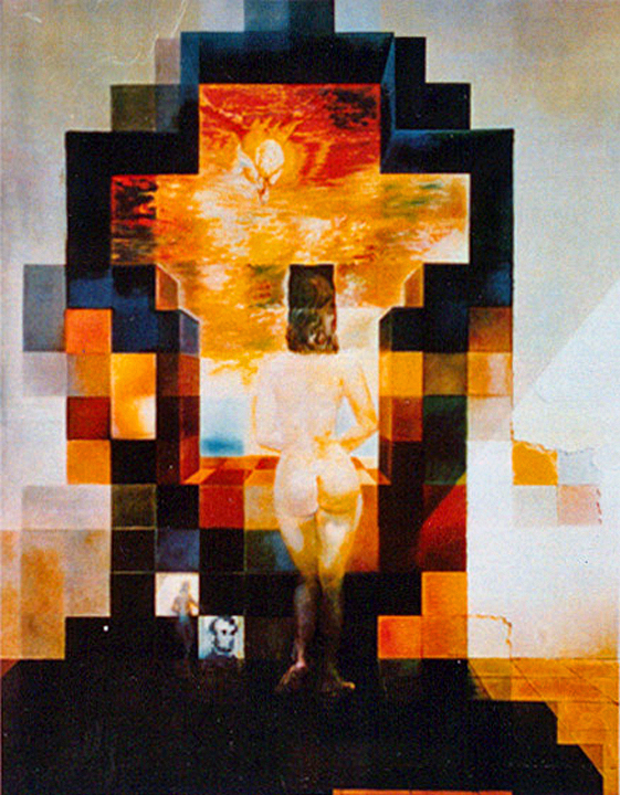
A gaussian stack of this image:


A laplacian stack of this image:
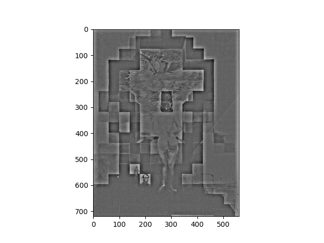
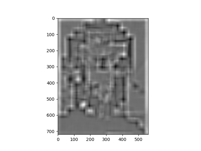

We can see that the details (including the woman) are visible in the high frequency bands of the laplacian stack but that Lincoln appears in the lower frequency bands.
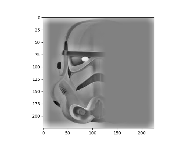
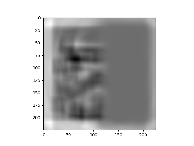
Applying these stacks to the picture using the koala and my friend Eric above we can see that the koala's face appears in the high frequences but Eric's face appears in the lower frequencies
A gaussian stack of this image:


A laplacian stack of this image:
We can use Gaussian and Laplacian stacks to blend two images together. To do this we represent the two images we want to use at different frequences using a laplacian stack for each image, then use a mask and the gaussian stack of that mask as the weights on each of the two source images. This technique is used on a few images below. For each we show the two source images and the final image.


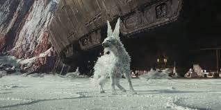
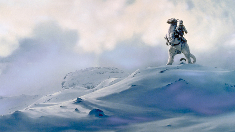
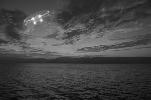
This technique can also be used on images where the combination boundary is not a straight vertical line, as illustrated in the images below.
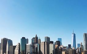
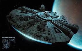
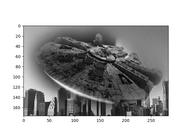
The approach does not work amazingly well, especially on the image of the Millenium Falcon and the city, because it only works on the edges of the image.
We can use the laplacian stack from above to illustrate the process by displaying the stack for the two source images and the combined image.


Instead of operating purely on the pixels of the image and using different filters to help blend them together, we can take an entirely different look at the problem of blending images together. We learned that human perception is more focused on gradients between pixels than on the absolute value of those pixels. We can set up an optimization problem seeks to pick values for pixels in the region of the target image such that their gradients are as close as possible to the source image. In this way we find values with gradients that are similar to the source and target images so that there are no sharp boundaries between the images. The least squares formulation of this optimization problem is below, with each '"i" as a pixel in the source "S" and each "j" is a four-neighbor of "i".

As a toy example, we set up a least squares problem to recover an image exactly from it's gradients, without involving a target image. The original image and the recovered version are displayed below.

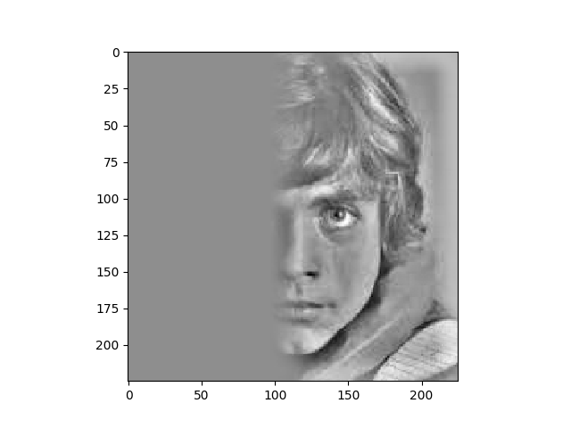
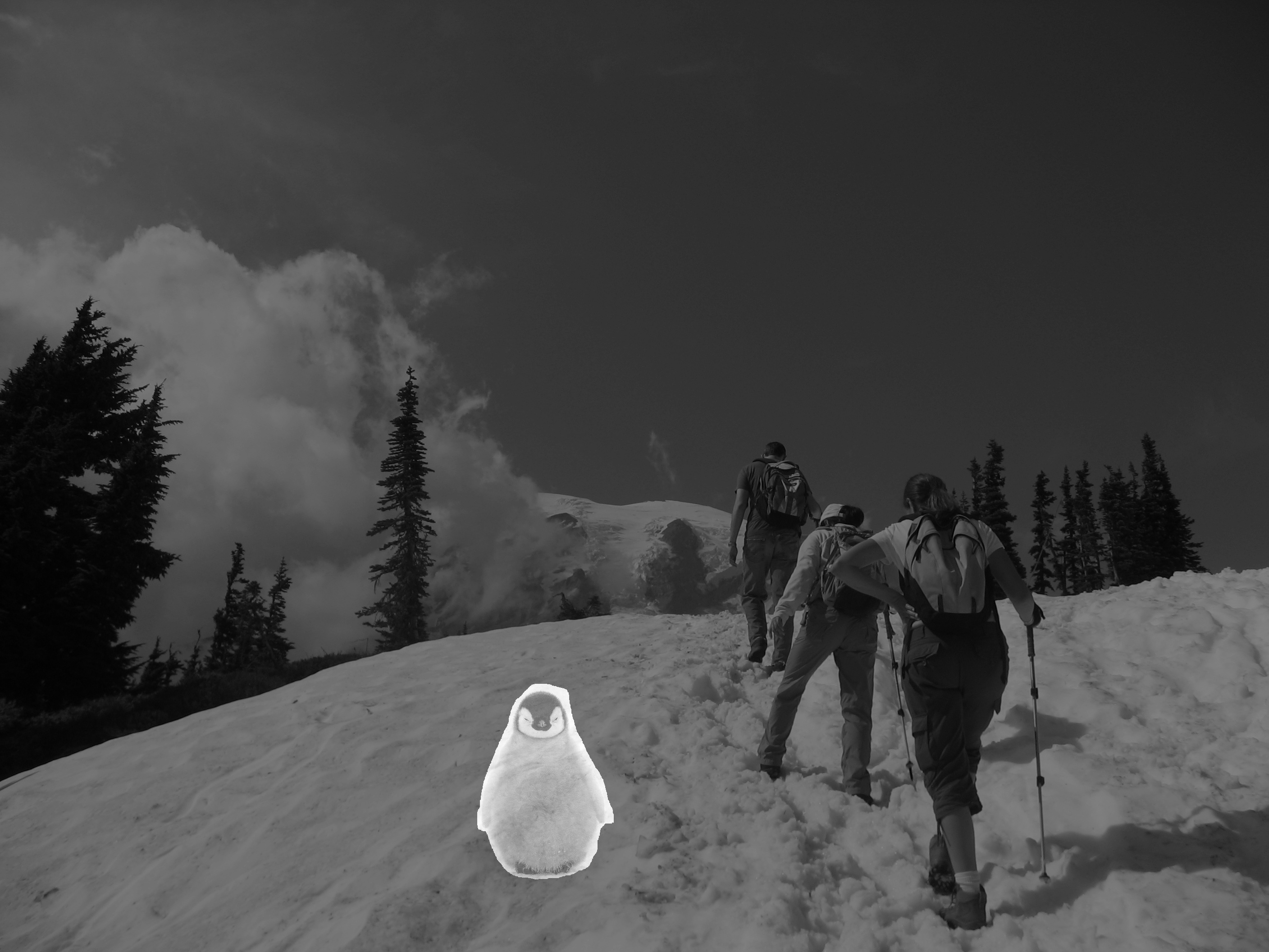
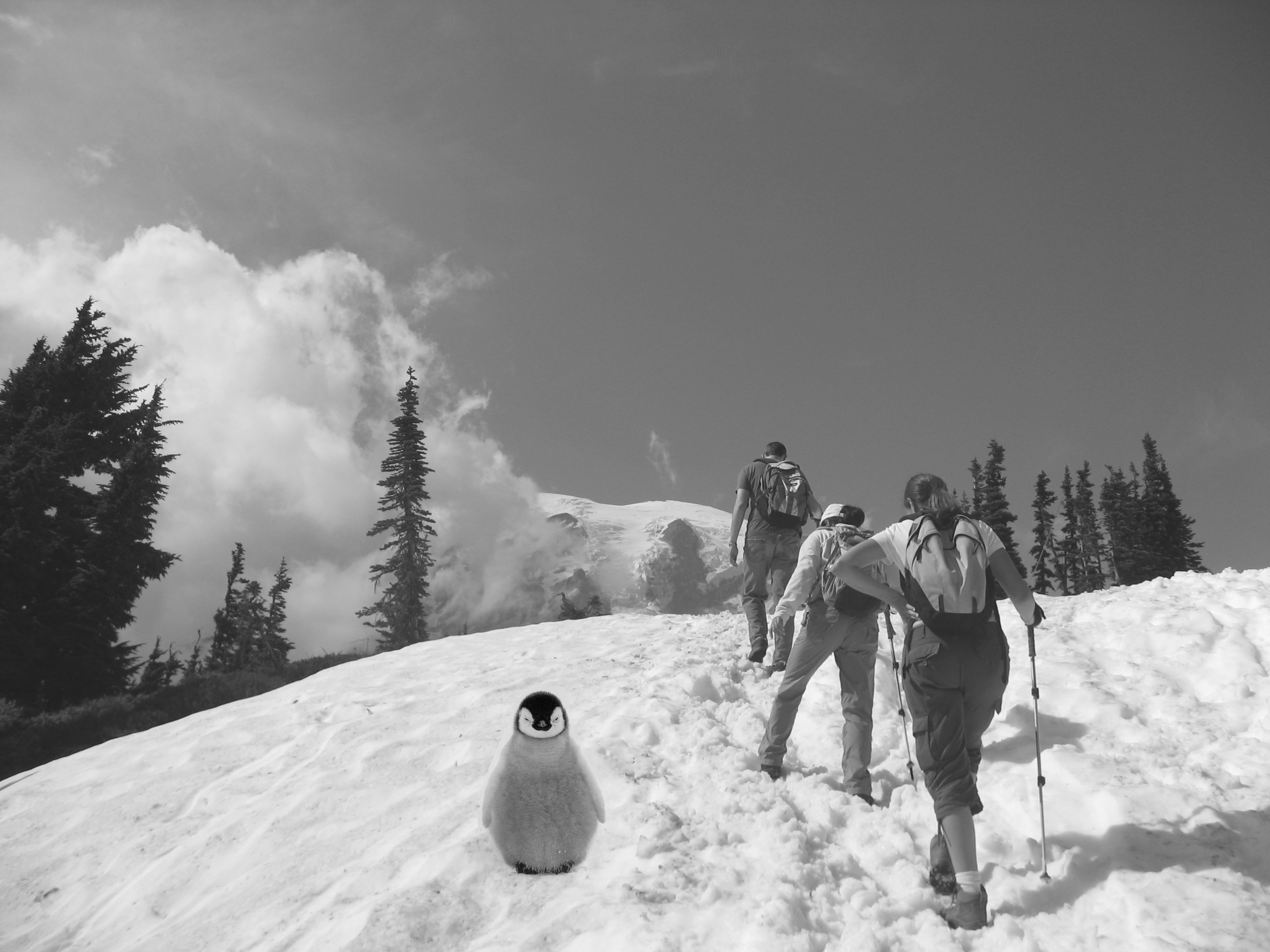
Building on the toy problem we set up the full optimization problem so that the gradients are dependent on both the source image and the target image. Results for several blending examples are below. For each example we show the source image, the target image, the result of naively copying the source image on top of the target image, and the final poisson-blended image.


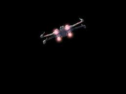
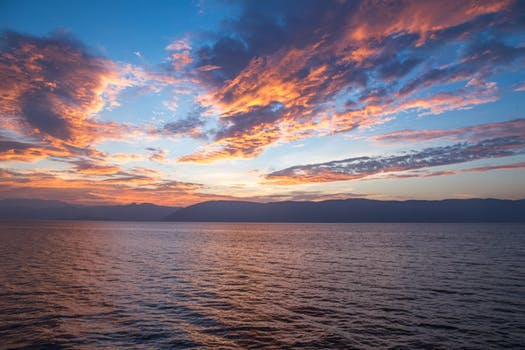

As seen above, poisson blending does not always produce the best results. In the case of the x-wing the backgorund is a very different color, and so the naive version seems to do better because the black background gets interpreted as a "0" value and so just the x-wing gets copied to the sunset. In the poisson version of this image the optimization creates a value that appears to be midway between black and the blue of the sky and so it looks more out of place.
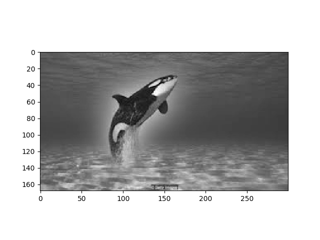
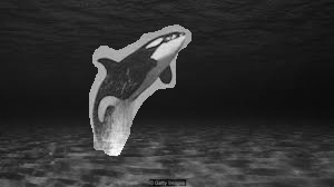
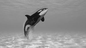
Similarly, I used the orca and ocean pictures in both the multiresolution blending part of the project and the poisson part. The multiresolution blending looks better for these two pictures because there is not a hard seam between the two images. In the poisson blending the backgrounds are sufficiently different from each other that it looks like there are some border artifacts around the orca.
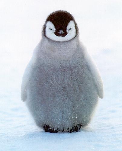
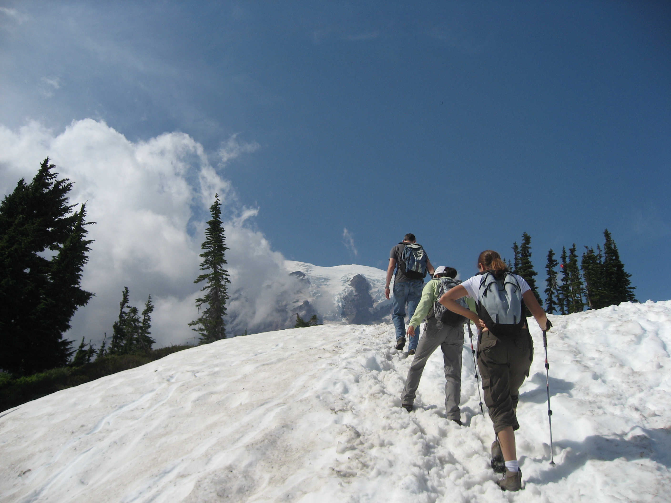
Poisson blending seems to work well when the background colors are sufficiently similar and there is not a lot of texture in the background of the source image, as seen in the penguin example and the ice fox example.