Part 1.1: Warmup
In this part, we are tasked with sharpening an image. We accomplish this by generating a Gaussian high-pass filter which contains the details of the image, by subtracting the low-pass filter from the image. We then add the high-pass filter back to the image to sharpen the image.
|
|
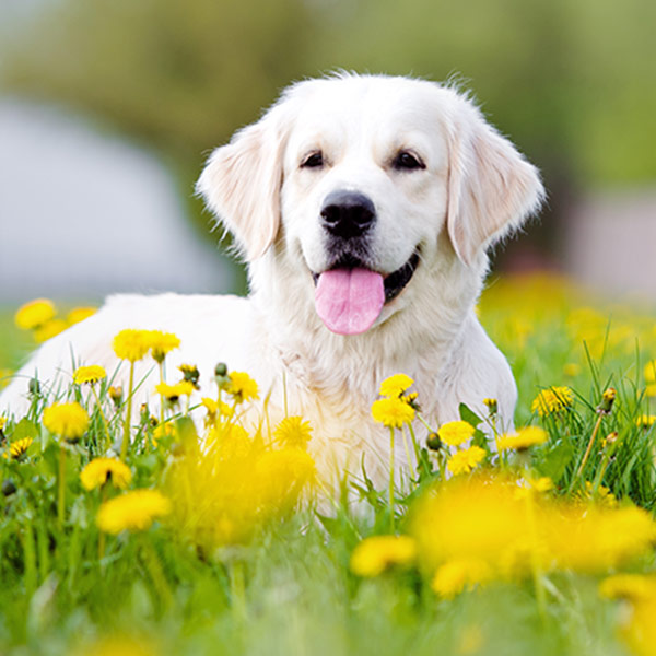
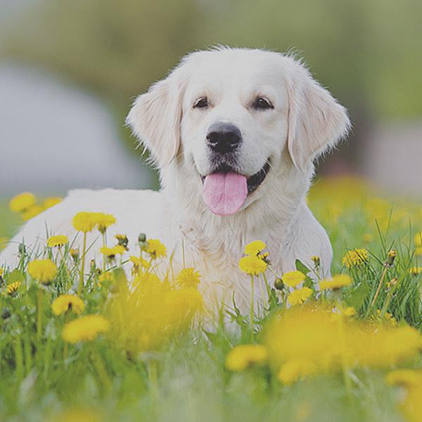
Part 1.2: Hybrid Images
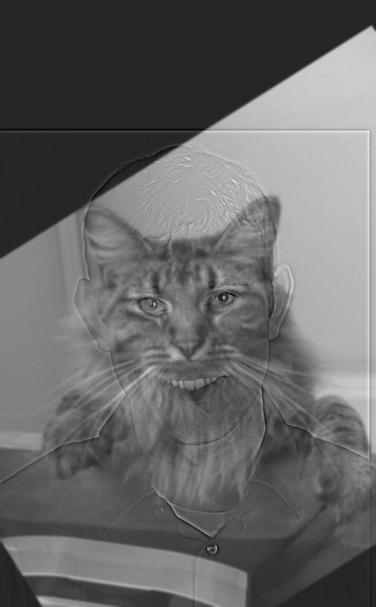
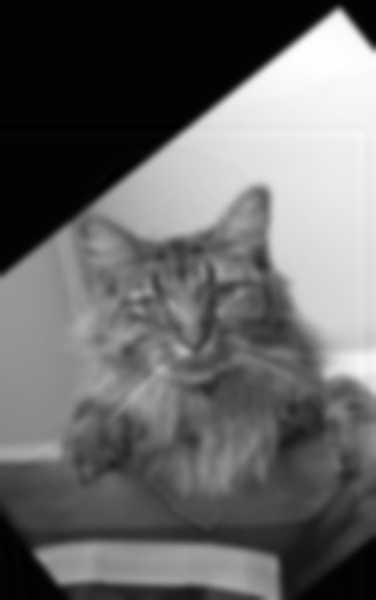
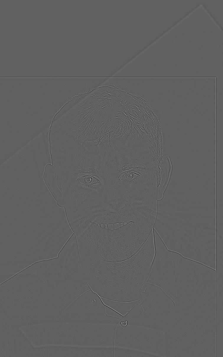
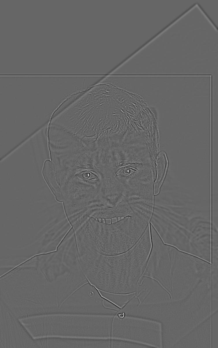
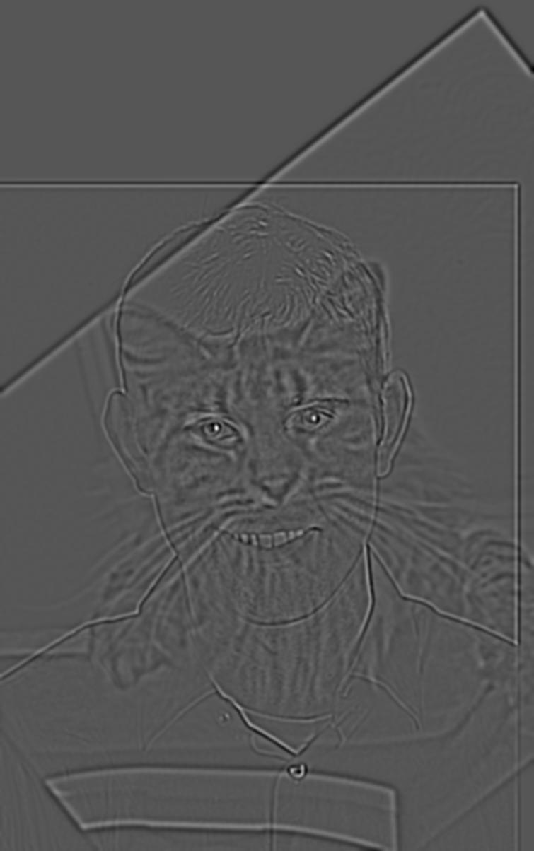
In this part, we are tasked with creating hybrid images, by combining the high-pass filter of one image with the low-pass filter of another. This creates an interesting visual effect: when close-up, you can more clearly discern the high-frequency details of the first image, but from afar, you are only able to see the broader lower frequences of the second image. Thus, the image appears to shift as you move in distance away from the image.
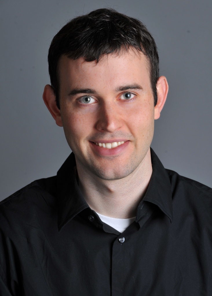
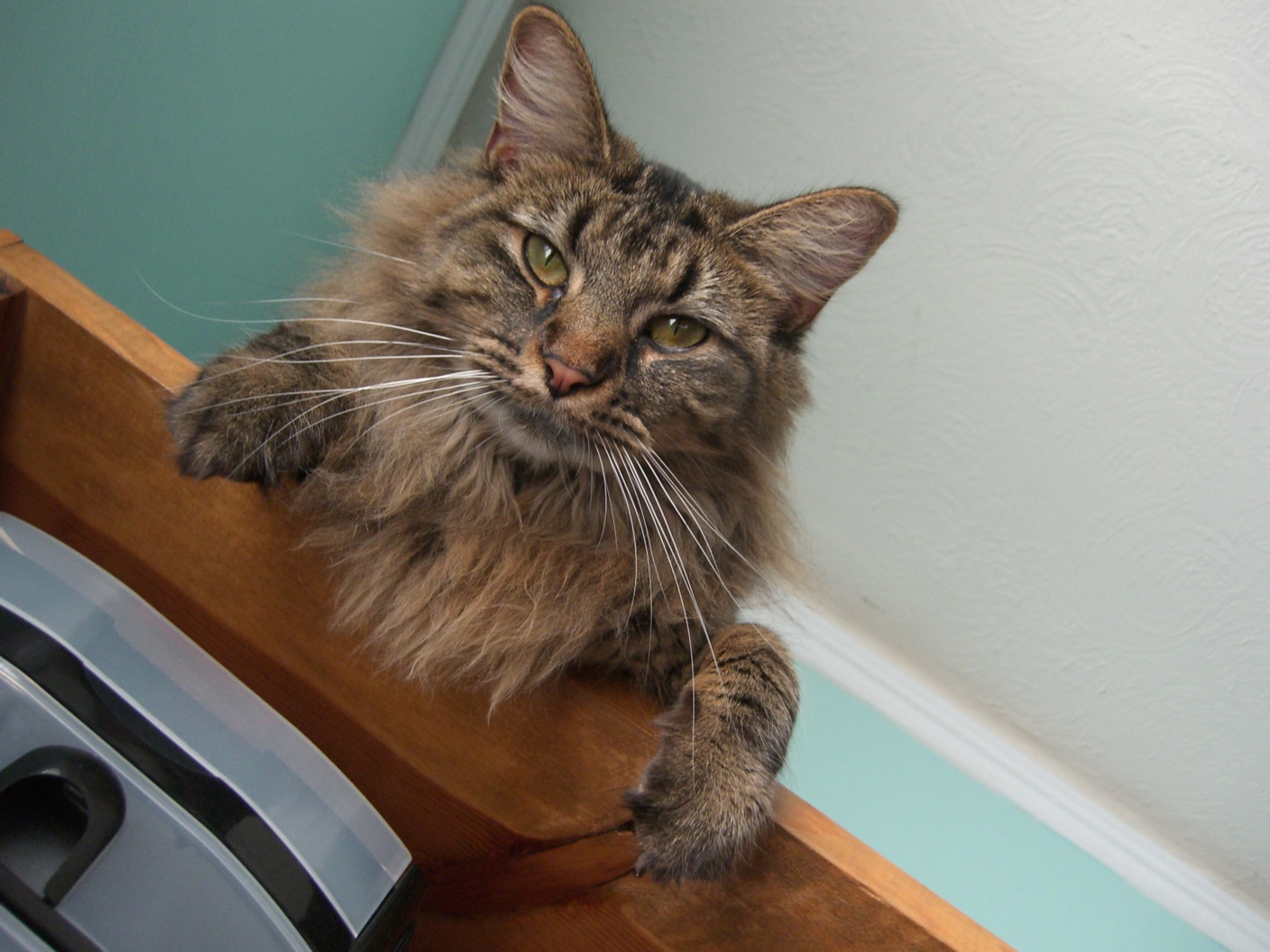
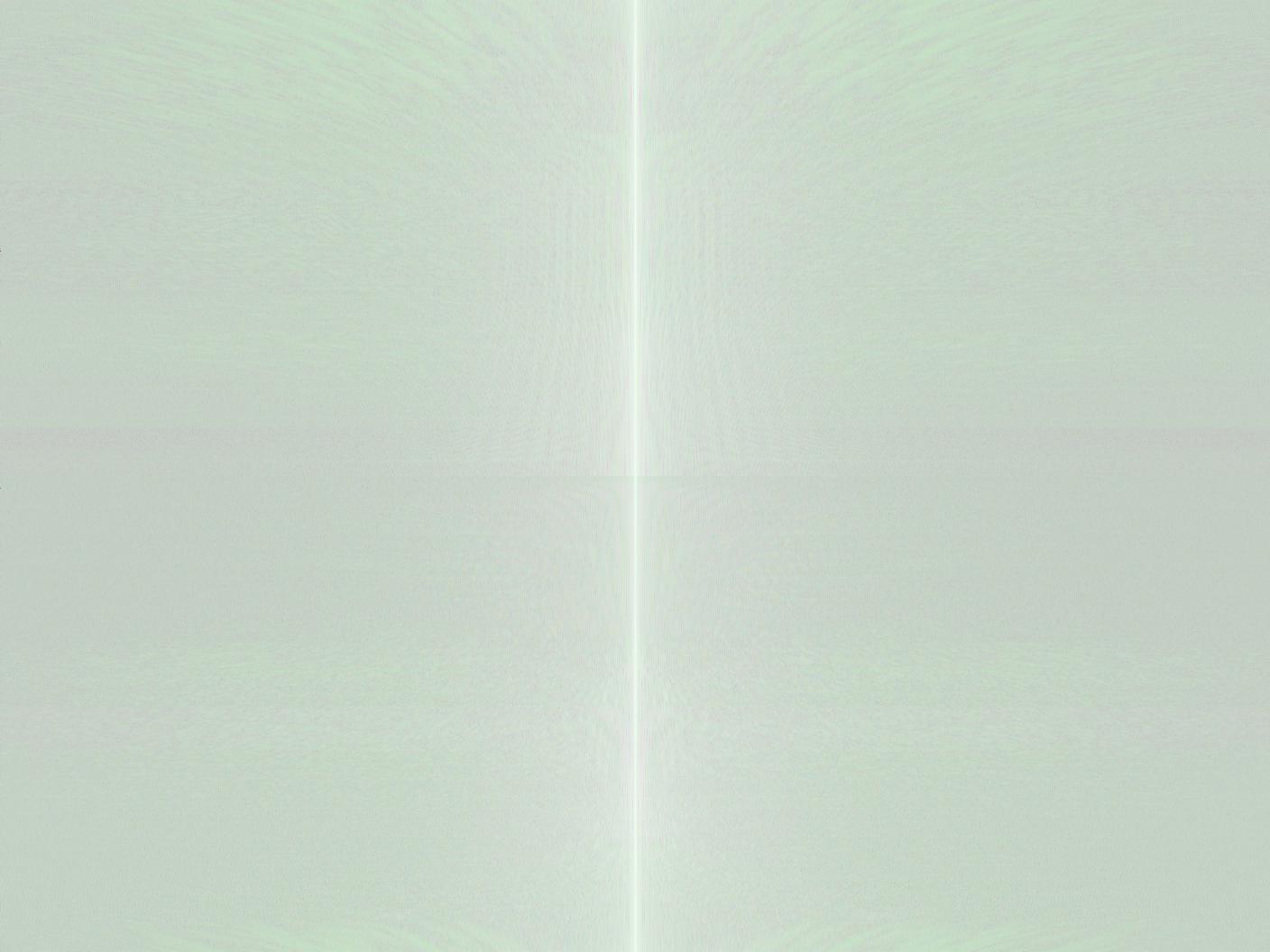
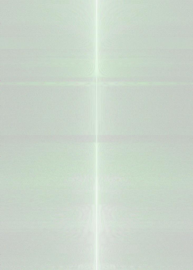
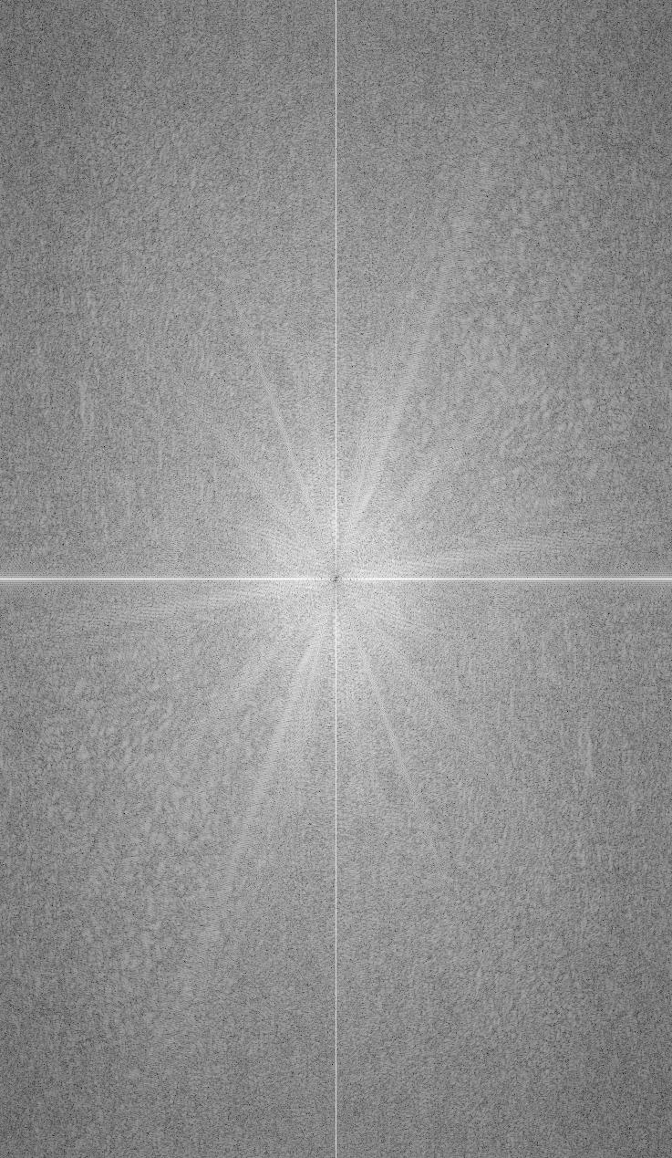
Nutmeg and Derek + FFT Analysis
|
|
|
|
| |
|
|
|
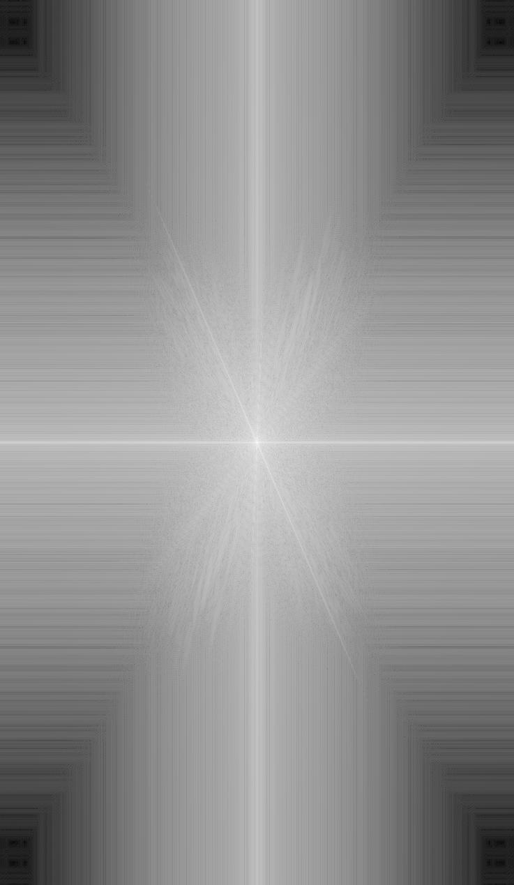
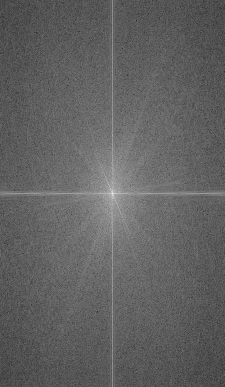
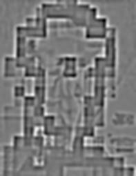
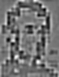
FFT Analysis
First, we notice that the high-pass FFT of Derek contained much more granular detail than the much blurrier low-pass FFT of Nutmeg. Both filtered FFTs, however, contained elements of their original images. Finally, we notice that the hybrid FFT contains features from both filtered images, including the granularity of the high-pass image, but also distinct features from the low-pass image.
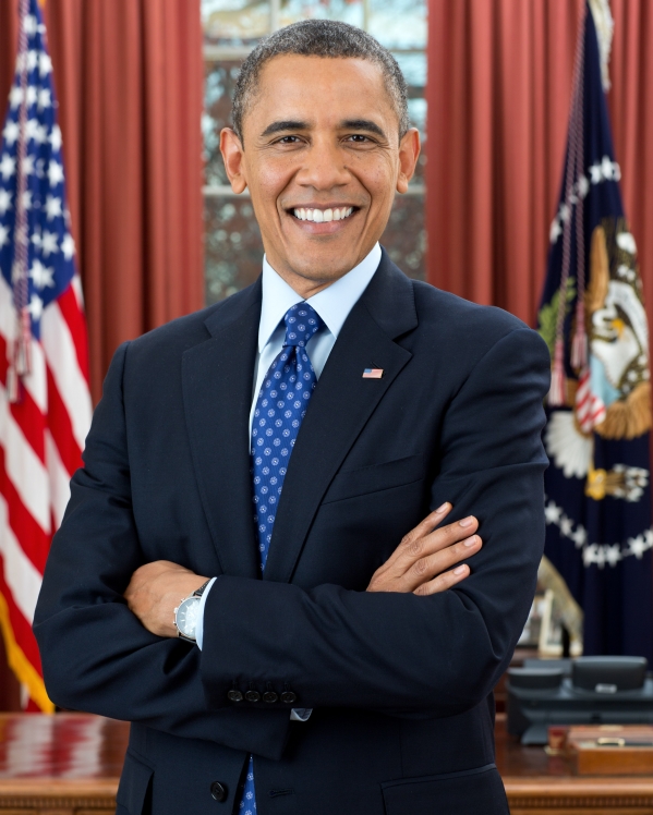
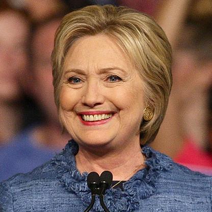
Obama + Clinton
|
|
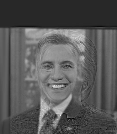
|
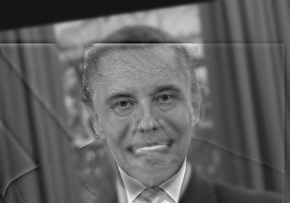
Obama + Trump (Failure Case)
|
|

|
|
This one was absolutely horrifying. This one did not work as well because the structure of the two faces were very similar, meaning that a lot of the differences between the two faces were blended together at all depths.
Part 1.3: Gaussian and Laplacian Stacks
In this section, we explore the creation of Gaussian and Laplacian stacks. Gaussian and Laplacian stacks allow us to store the individual frequency slices of images, which allow for multiresolution blending (as seen in part 1.4).
Unlike a pyramid, each slide in the Gaussian stack has the same dimensions, but with differing levels of sharpness. This is done by adjusting the parameters of the Gaussian kernel. The first image of the Gaussian stack is the original image, and the slides then decrease in frequency.
The Laplacian stack holds the frequency difference between consecutive images in the Gaussian slack. The first slide (L0), is calculated by the difference between the first and second slides of the Gaussian stack (G0-G1). The last slide of the Laplacian stack is simply the last slide of the Gaussian stack.
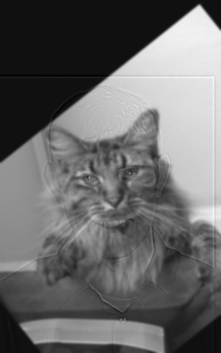
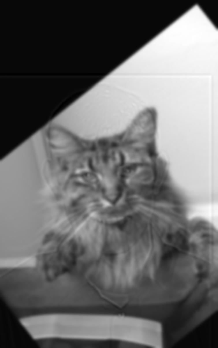
Nutmeg + Derek hybrid

|

|
|
|
|
|
|
|
|

|
Because the Gaussian steadily loses frequency with each slide, we observe the low-frequency image becoming steadily more apparent. Likewise, with the Laplacian stack, we see the increasing appearance of the low-frequency image with each slide.
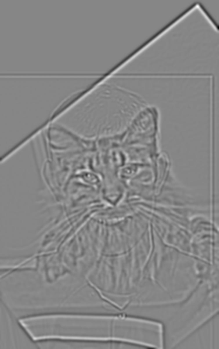
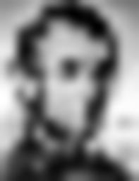
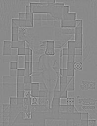
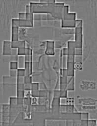
Dali Lincoln Painting

|

|

|

|
|
|
|
|
|

|
Because this painting contains different details at different frequencies, we see the Gaussian stack steadily losing higher-frequency deteails, while the Laplacian stack shows the different details between different frequencies.
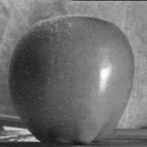
Part 1.4: Multiresolution Blending
In this part, we utilize the Gaussian and Laplacian stacks to perform multiresolution blending. We blend two images across multiple layers (with a pre-defined blending mask), by first starting with the lowest-frequency Laplacian and Gaussian slides, and gradually blending increasingly higher-frequency layers. We use the provided logic for blending, where Ga represents the Gaussian stack of a blending mask, and LX, LY are the corresponding Laplacian stacks from the same image:
LBlend(i,j) = Ga(l,j)*LX(l,j) + (1-Ga(I,j))*LY(I,j)
Orange + Apple

|

|

|
|
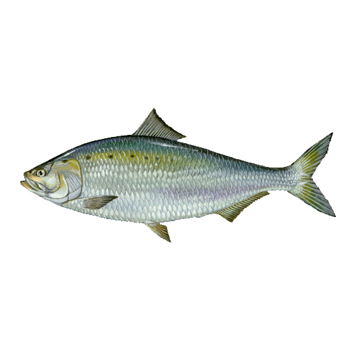
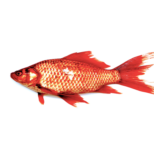
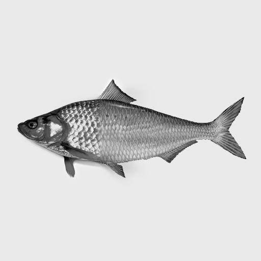
Fish + Fish
|
|

|
|
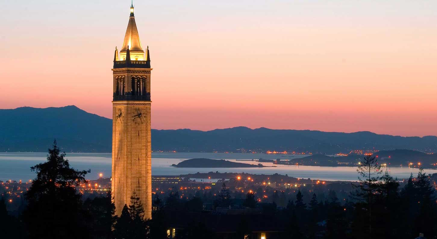
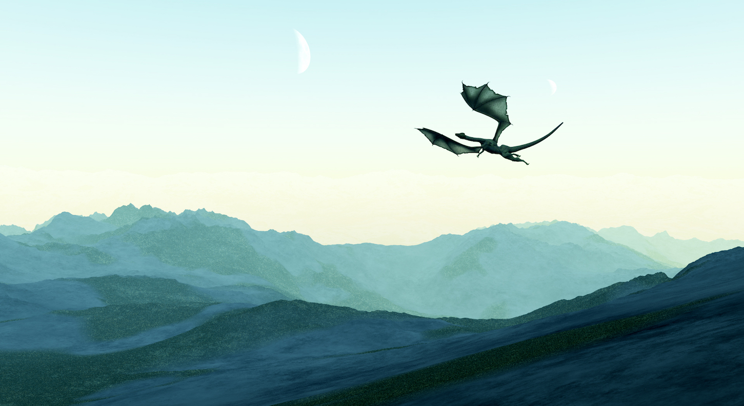
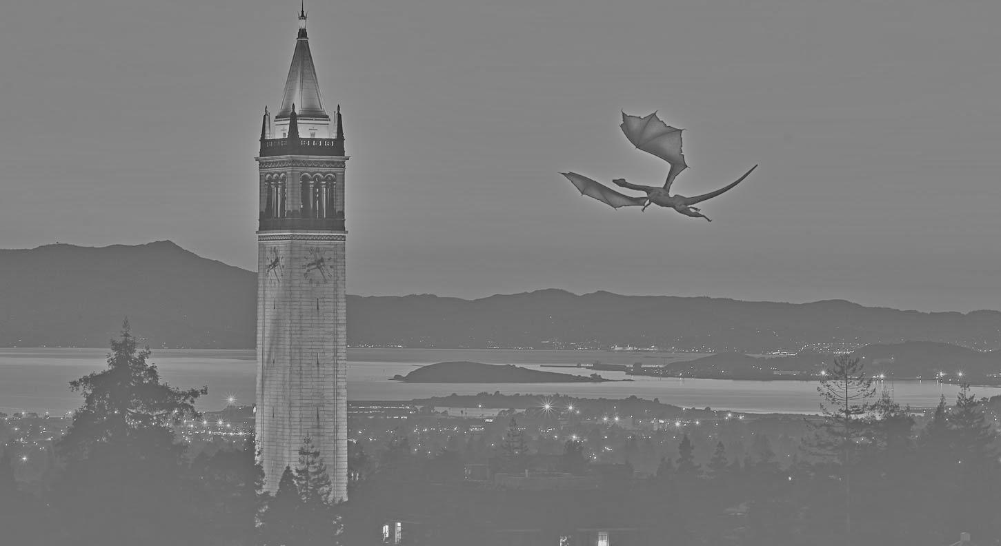
Dragon in Berkeley (Irregular)
|
|
|
|
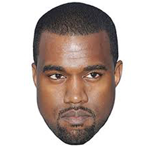
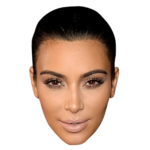
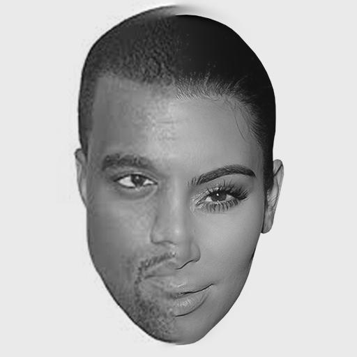
Kim and Kanye (failure case)
|
|

|
|
This one did not come out as well because their faces did not line up exactly, and they had difference in shapes for each respective facial feature.
Part 2: Gradient domain fusion
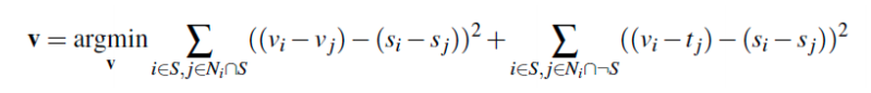
In this part of the project, we explore another way of manipulating images. Using gradient domains, we can preserve gradiants between pixels of the original image, allowing us to fuse one region of an image into another one and have it blend in seamleslly. The new pixels take on the color profile of the surrounding target image. In the process of moving region S to target T, we compute the gradient for each pixel in masked area S and its four adjacent neighbors. For pixels outside of region S, we simply use the gradient of T for that pixel. We use the following provided Least Squares Differerence to solve for the gradient, which we represent using a linear system of A, a sparse matrix, v, the solution vector representing the gradients, and b, the relative intensities in the final image:
Part 2.1: Toy problem
In this part, we utilize gradient domains to reconstruct an entire image. We compute the gradients for an image in the x and y directional derivatives, and then set the upper left most pixel to be equal. This ensures that when reconstructing the image, the gradients are placed in the correct location. By solving a similar linear system as above, our solution vector represents an almost-identical version of the initial image, built using the gradients alone.
|

|
As you can see, the reconstructed image is nearly identical to the original.
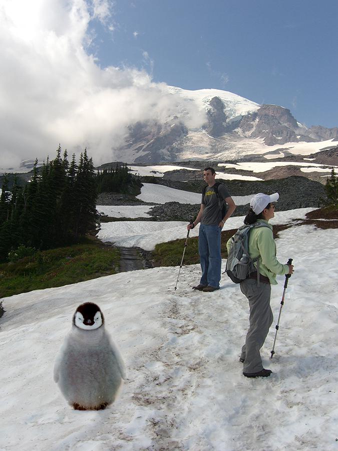
Part 2.2: Poisson blending
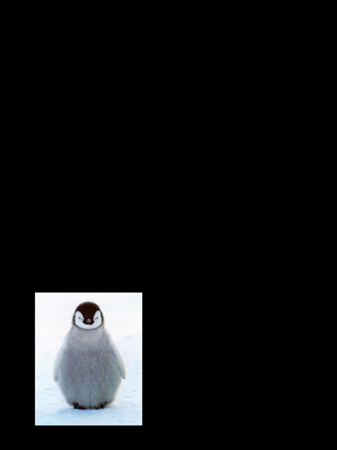
In this part, we implement the linear system described above. First, we computed the solution vector v, representing the gradients of our selected source image area. We then patched this gradient onto our target image to create the blended results.
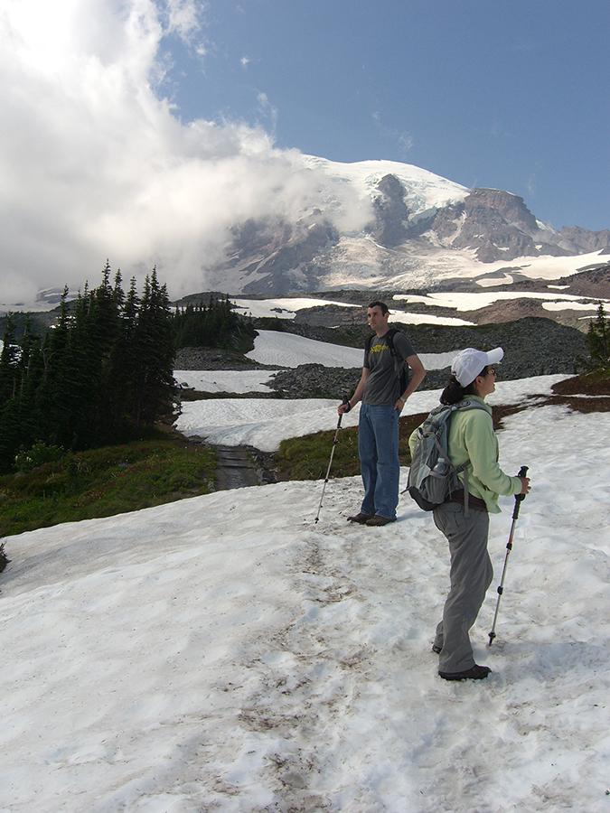
Penguin and Snow example
|
|
|
|
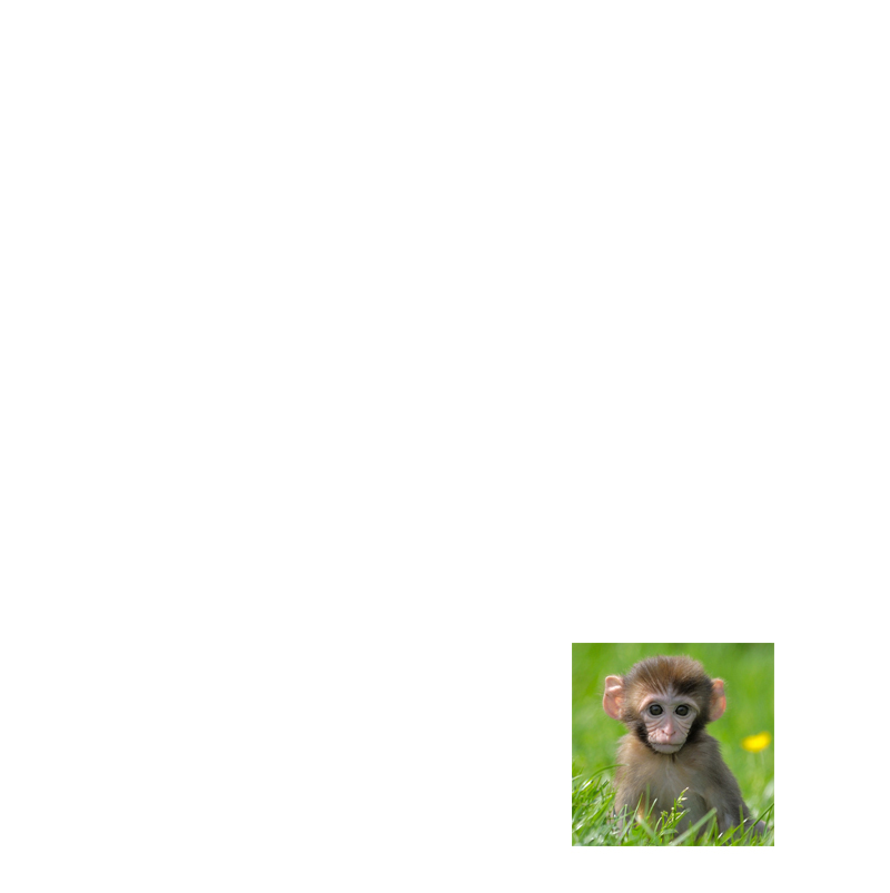
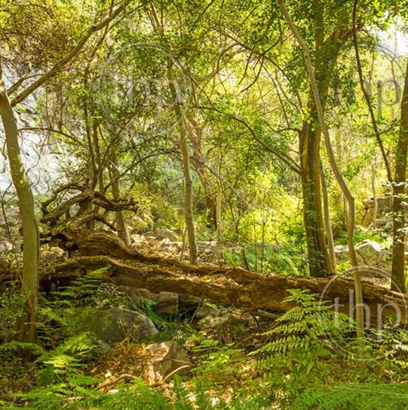
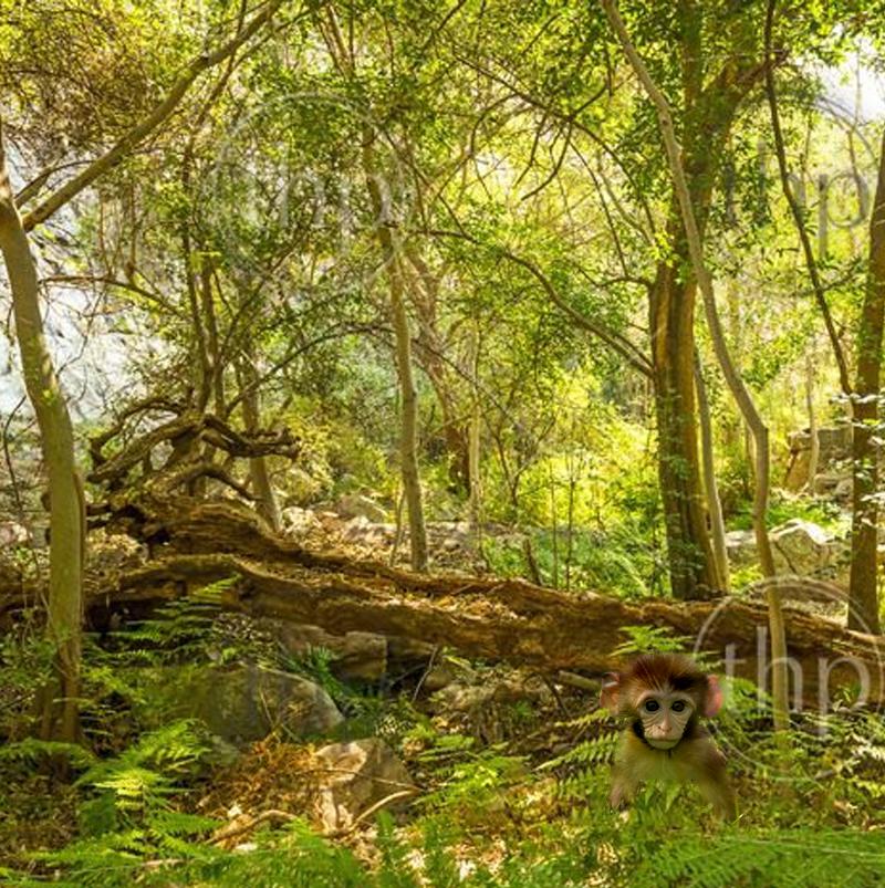
Monkey in jungle
My favorite is one in which I blended sitting on grass into the jungle, his natural habitat. This was my favorite because of how well it turned out.
|
|
|
|
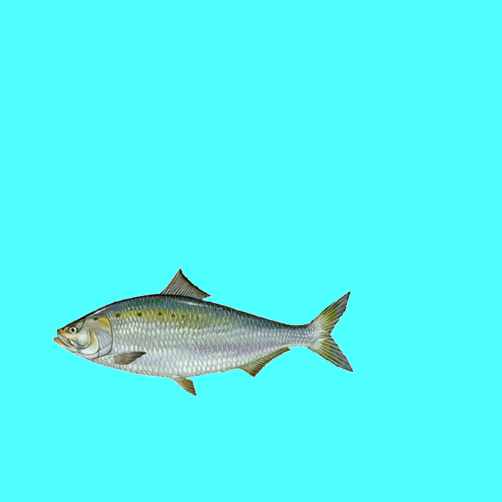
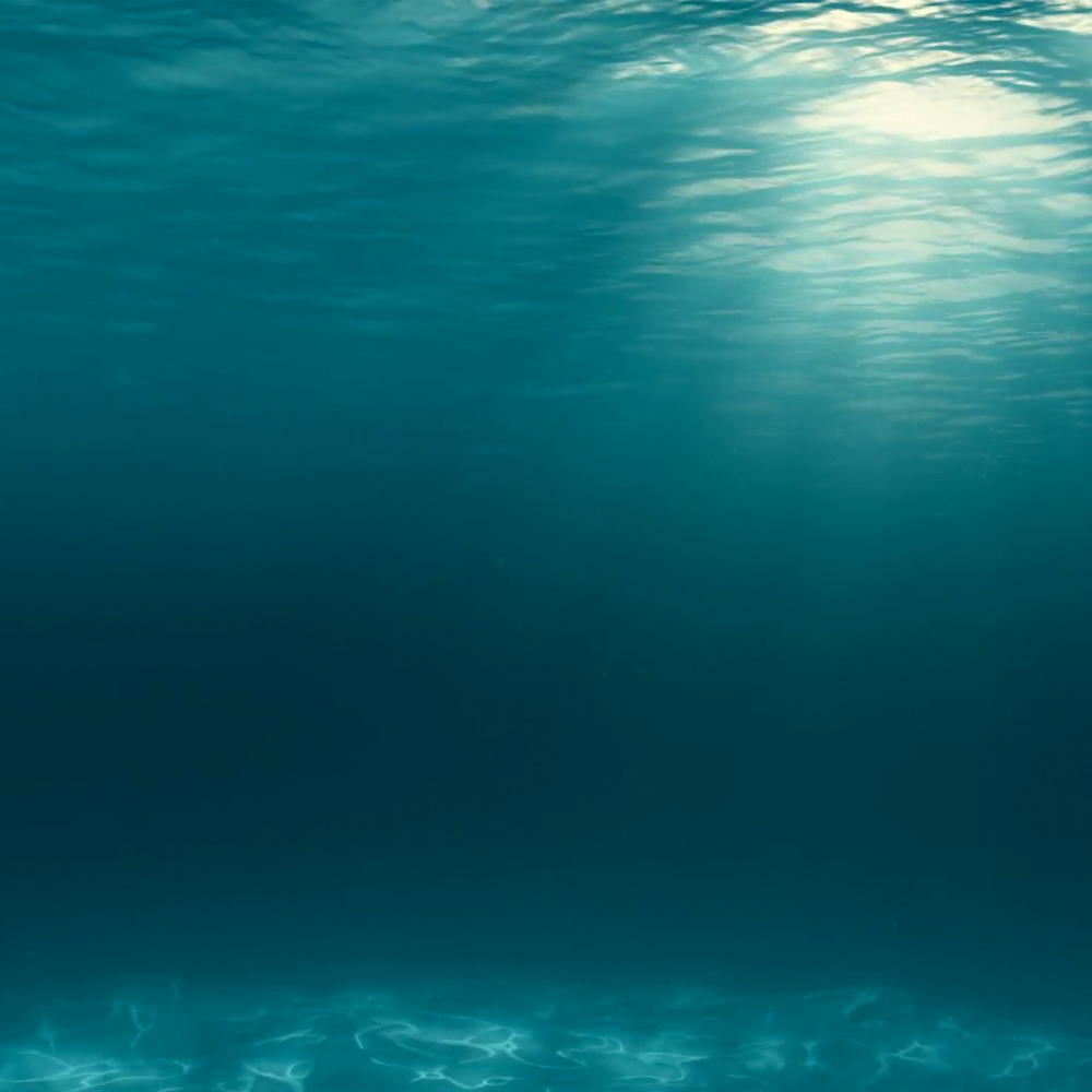
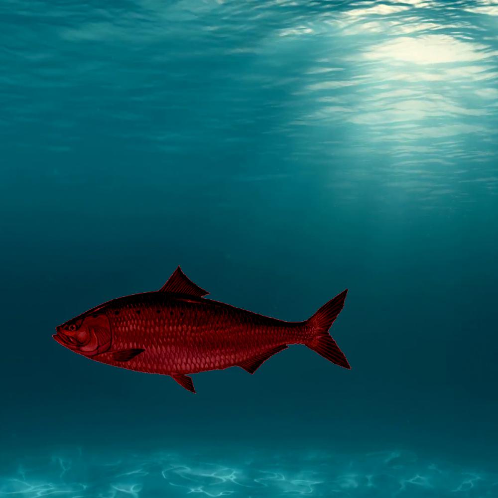
Fish in the ocean (Failure case)
|
|
|
|
This one didn't seem to work as well, because there was significant discoloration of the fish. I think this happened because the background color of the fish contrasted too heavily with the surrounding area, and my mask was not particularling tight, leading to a lot of noise in the eventual gradient from the source background.
Comparison to previous blend
I compared the Dragon in Berkeley multiresolution blend to a poisson blend.
|
|
|
Destination, Source, and mask |
|
|
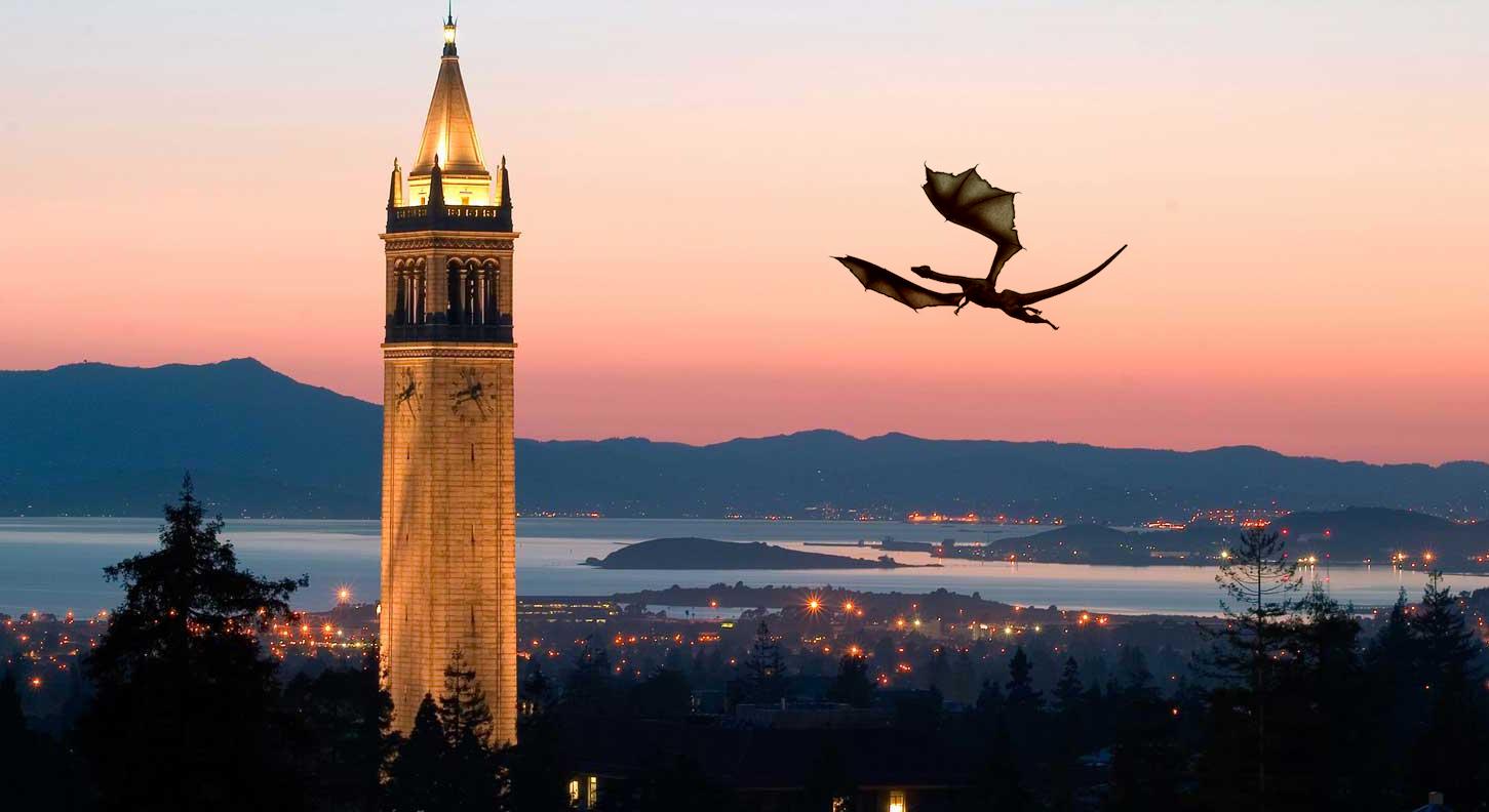
Multiresolution blend (first), Poisson blend (second) |
Both results actually work very well, although it is difficult to compare them because the first blend was not in color. I was very happy with the way that the poisson blend correctly blended in the dragon's surroundings. In general, I think the multiresolution blend is good for blending two seperate objects, with jarring seams, into on object. Meanwhile, the Poisson blend is better for putting objects in one setting into another one seamlessly.