|
|
|
The purpose of this project was to explore the applications of applying different transforms to images. We focused on the specific application of stitching images together in a panorama/mosaic fashion. To do this we took images and found homographies to project them onto some plane. A process that can also be used for image rectification, this allowed us to project images onto the same space and use blending tactics like linear and laplacian blending to blend images together to create a lovely panorama or mosaic.
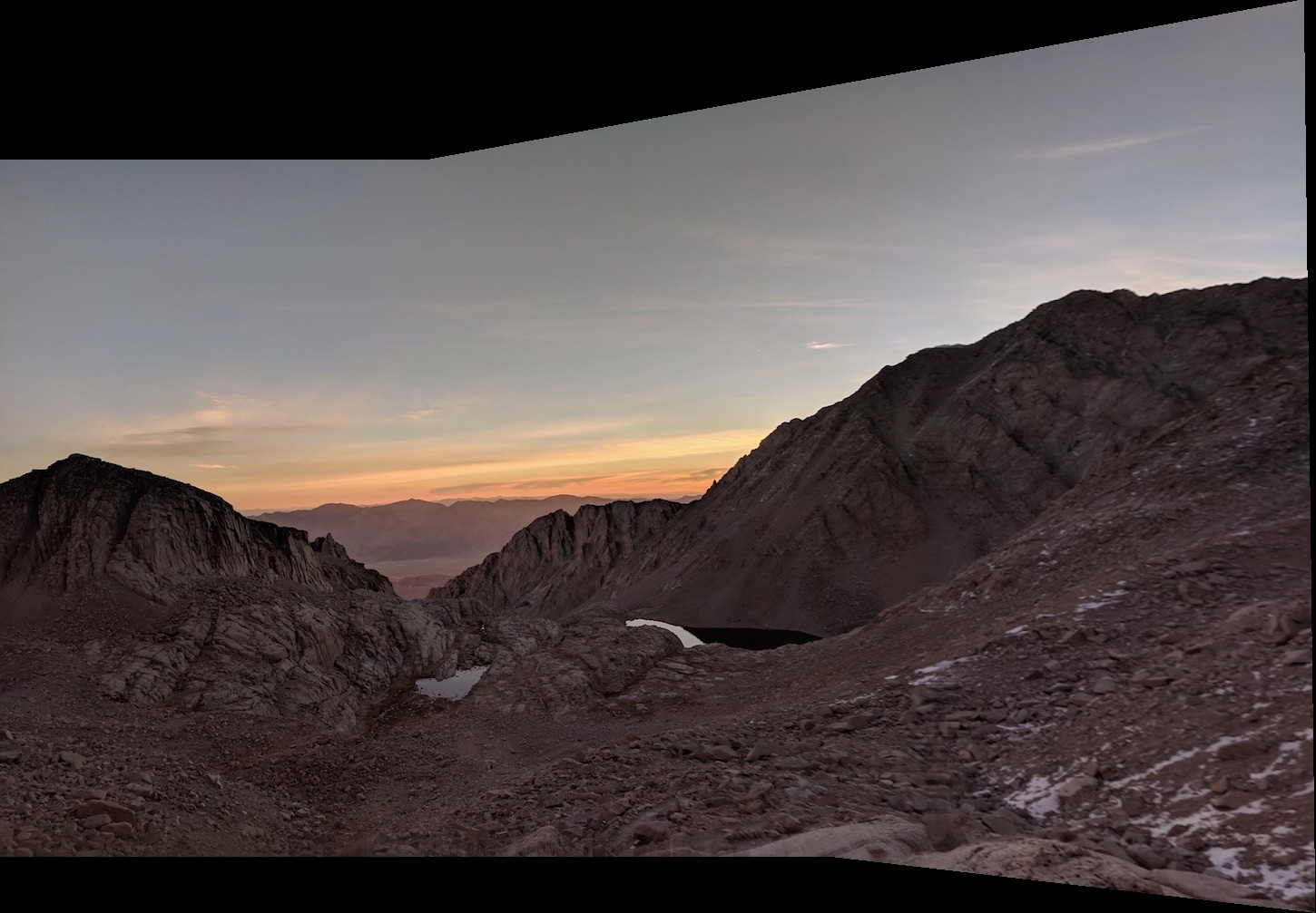
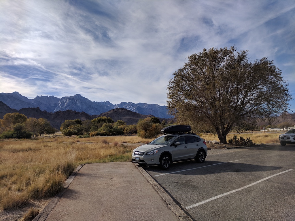
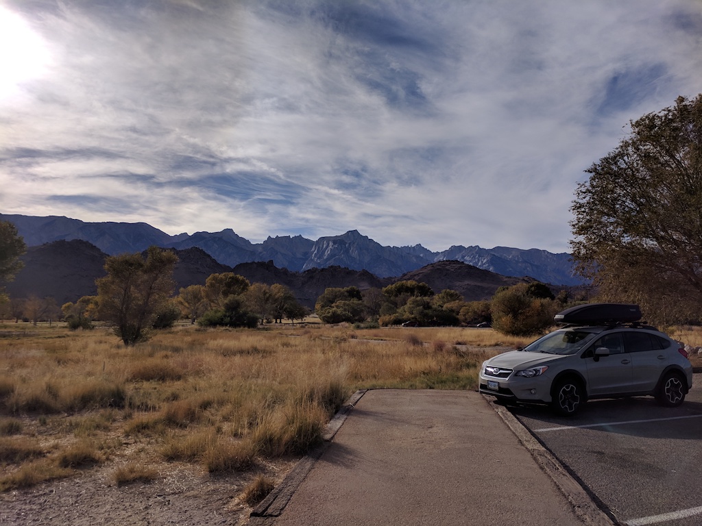
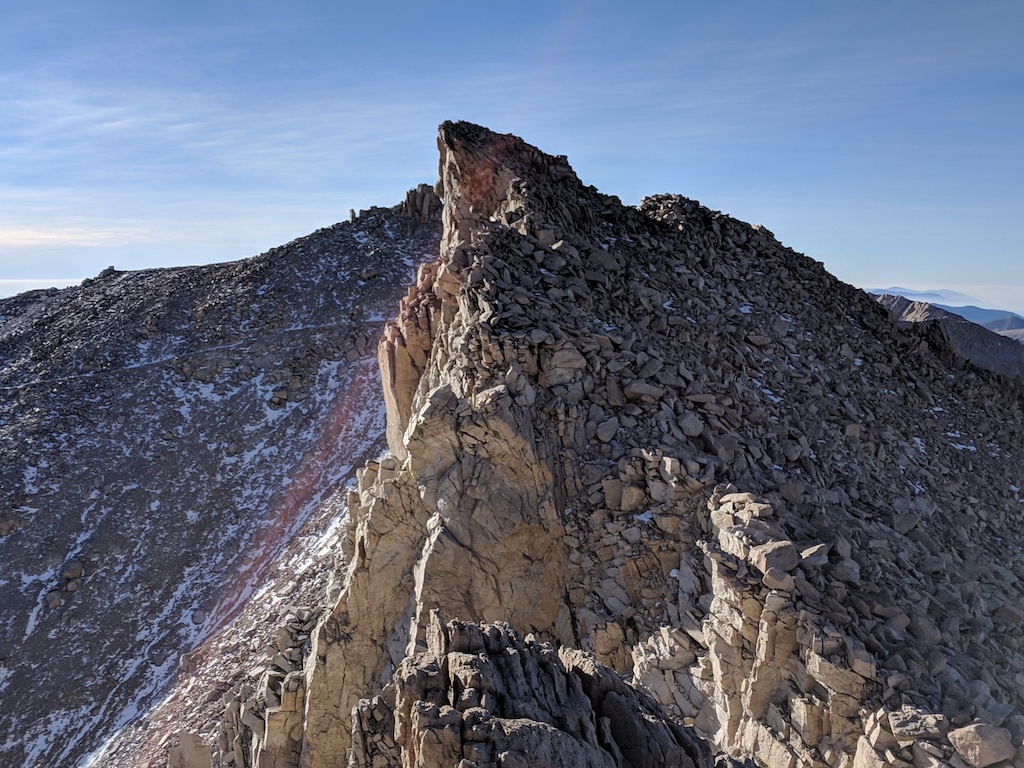
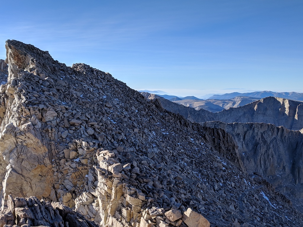
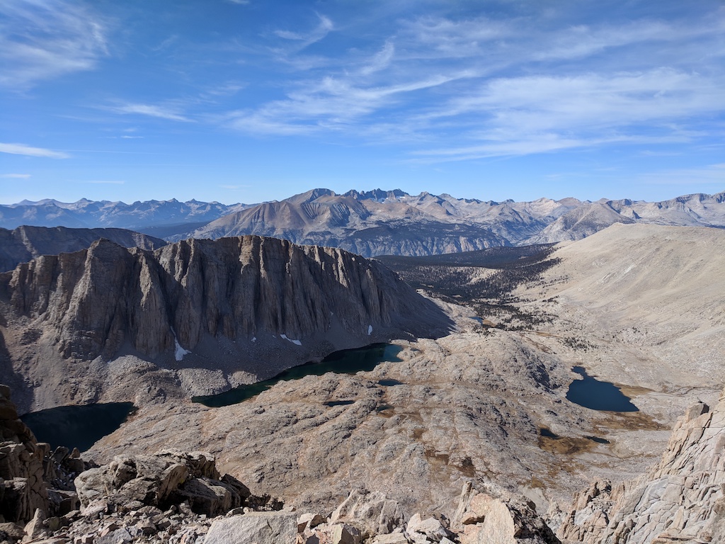
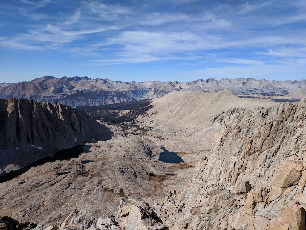
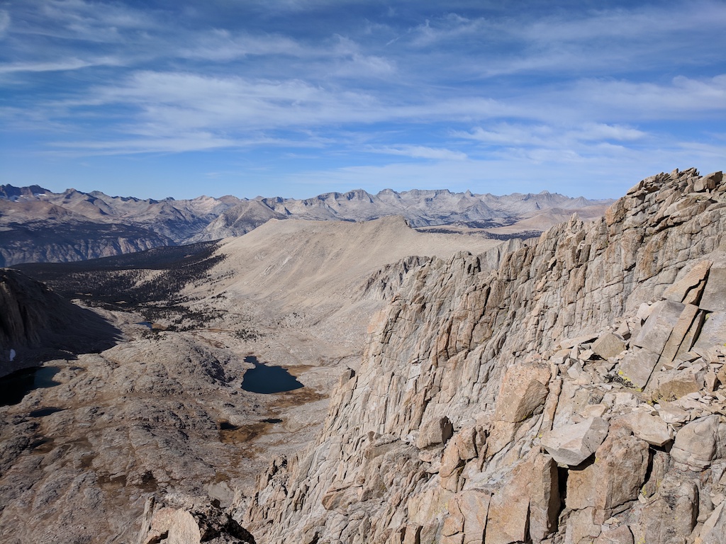
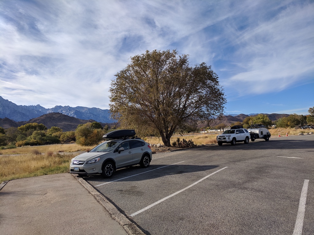
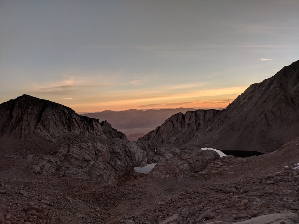
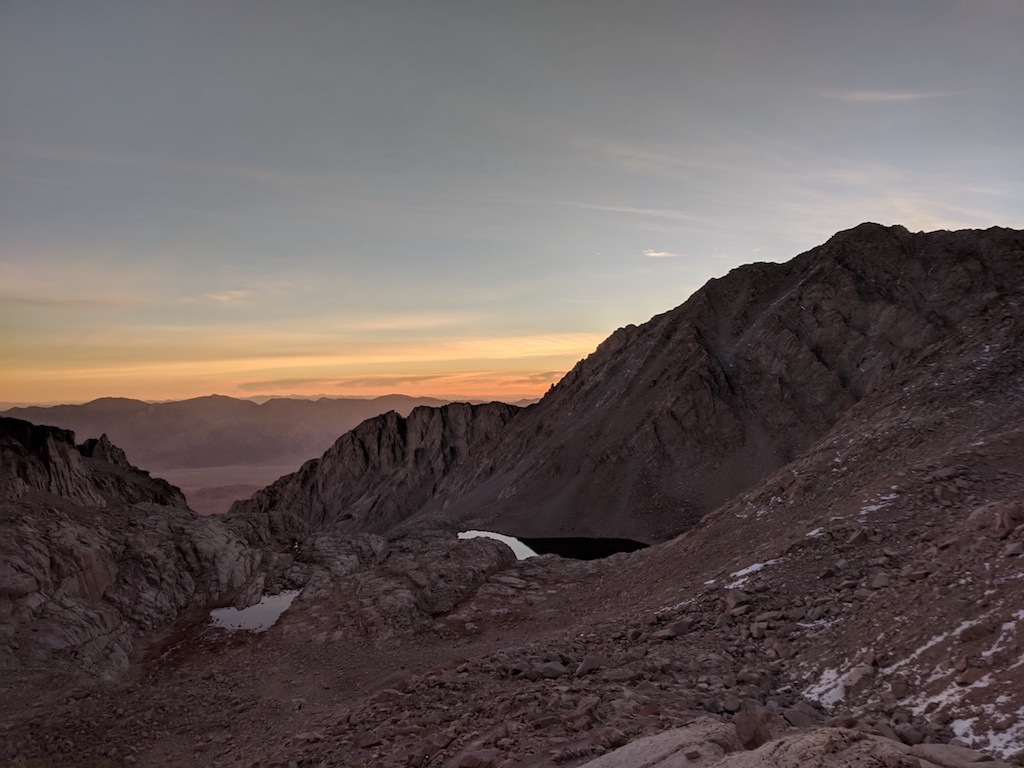
All the pictures displayed in this project were shot using a Google Pixel XL smartphone by me: Nikhil Uday Shinde other than the image labeled paper with scissors which was taken from a google search. For mosaics the camera was held still in hand and rotated about a point with significant overlap between the scenes captured. This allowed for the images to appear as though they were taken from approximately the same point with the difference being accounted from only the angle that the camera was facing. By photographing the images like this we see better results for the homographies that are used for the projections to generate the panorama.
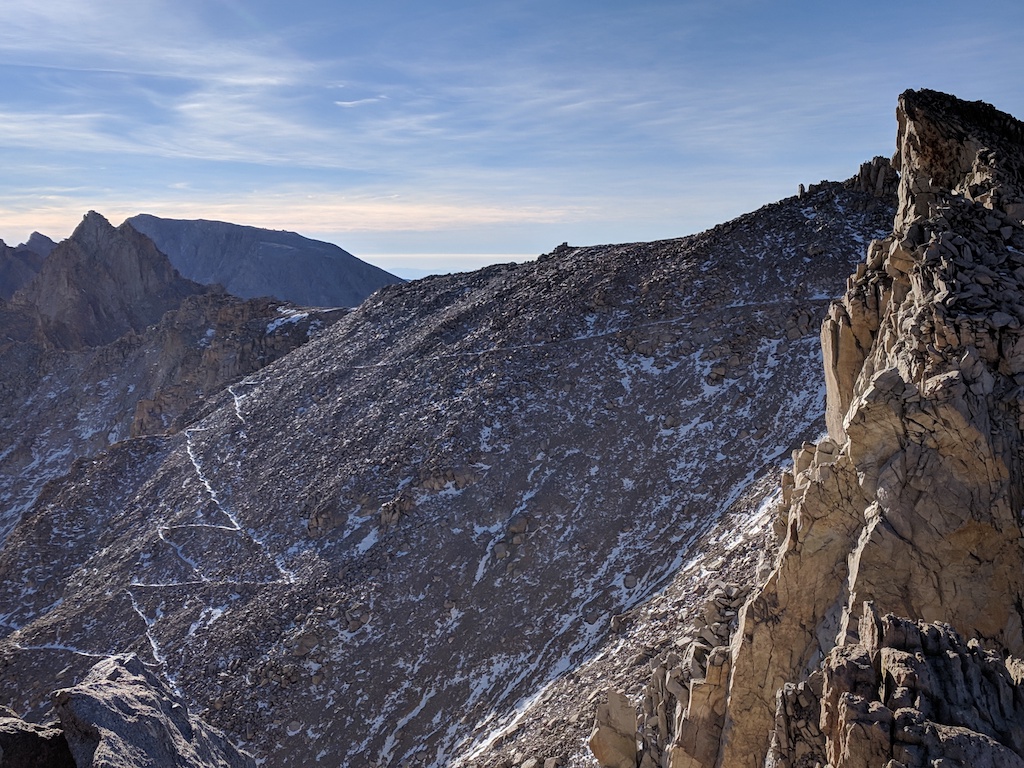
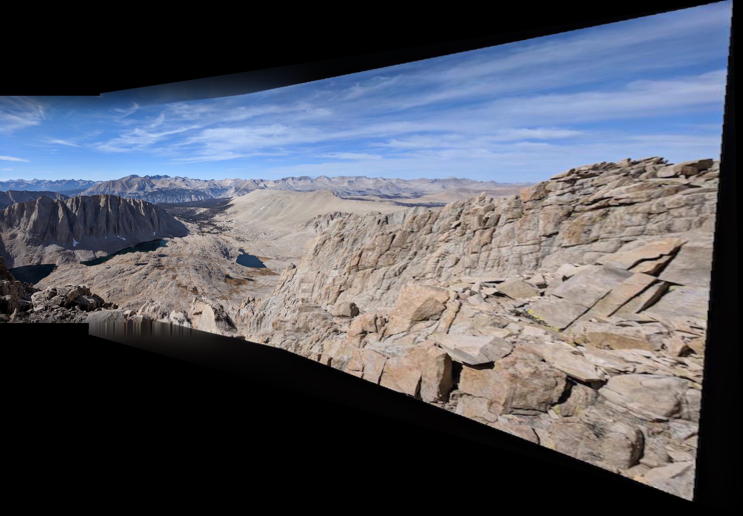
Fun fact: All mosaic images were shot on a weekend trip to climb Mount Whitney the tallest mountain in the contiguous United States/Lower 48!
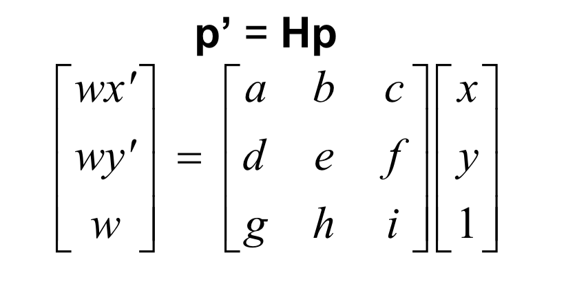
To start the process of creating the panorama we find transform that can warp the image. This allows us to rectify or warp one image to another making it easier for us to blend images together into a panorama as they are transformed onto the same plane. In order to accomplish this we solve for the following transformation or homography matrix (image credited to cs194-26 slides:
|
In order to do this we have to select the initial points on the image we want to transform and either select or specify corresponding points for them to transform to. Once this is done we use these points to construct the following matrix:
|
Now that we have found the homography matrix we can warp our image. To do this we adopt the inverse warp method we utilized in project 4. We first use the forward homography on the corners of the image to establish bounds of the target image. Then we use the inverse transform on each pixel in the target image to find which pixel value of the original image it should correspond to. We can then use an interpolation function to fill out these pixel values and construct the warped image. In fact all these computations can be done using a matrix multiplication and some vectorization!
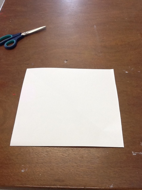
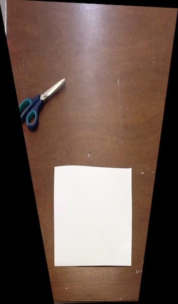
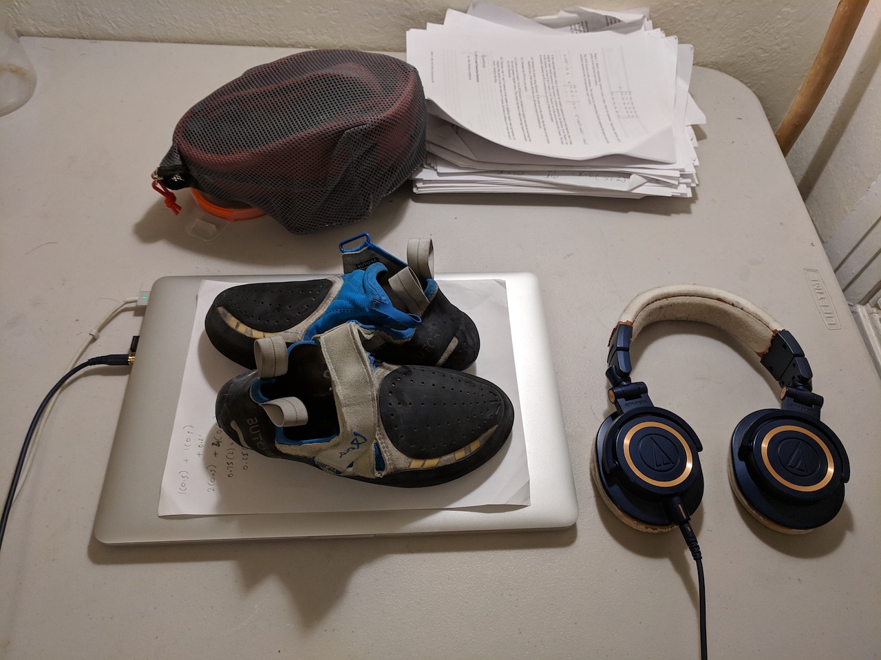
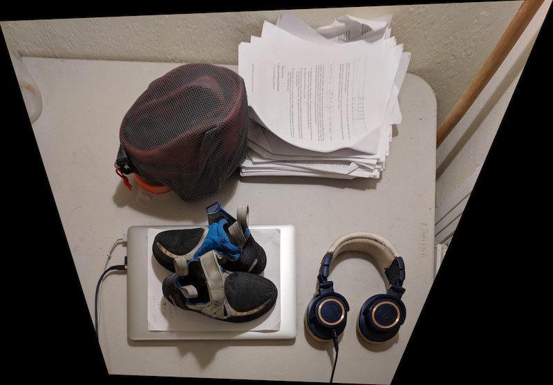
We can use the warp defined above to transform images such as they appear to be viewed from a different perspective. The following images were taken looking at objects on/near pieces of paper from a side angle view. By choosing the appropriate points in the initial image and appropriate corresponding points for them to map to we can compute a transform that generates a different perspective on the object, or a rectified view.
|
|
|
|
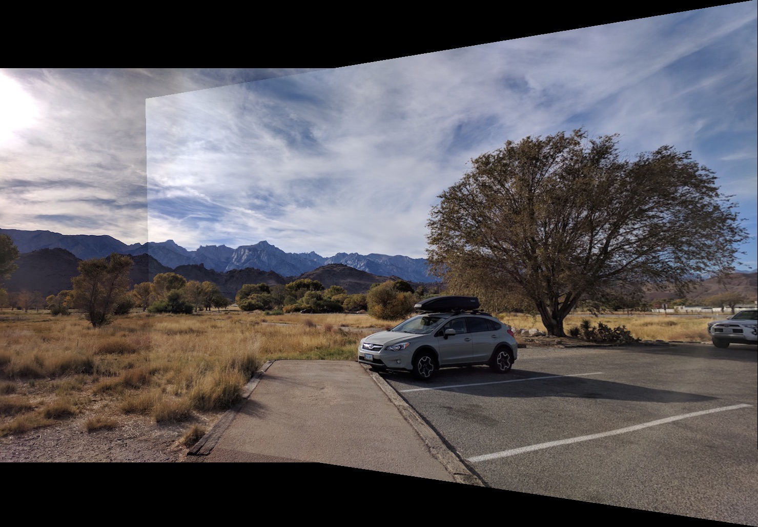
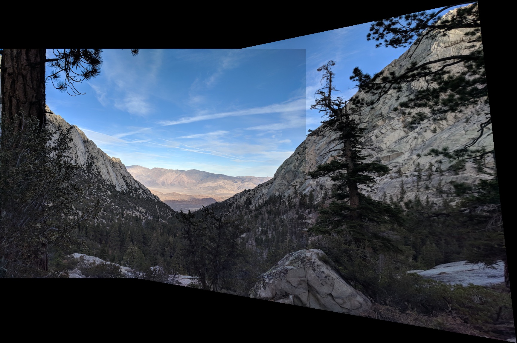
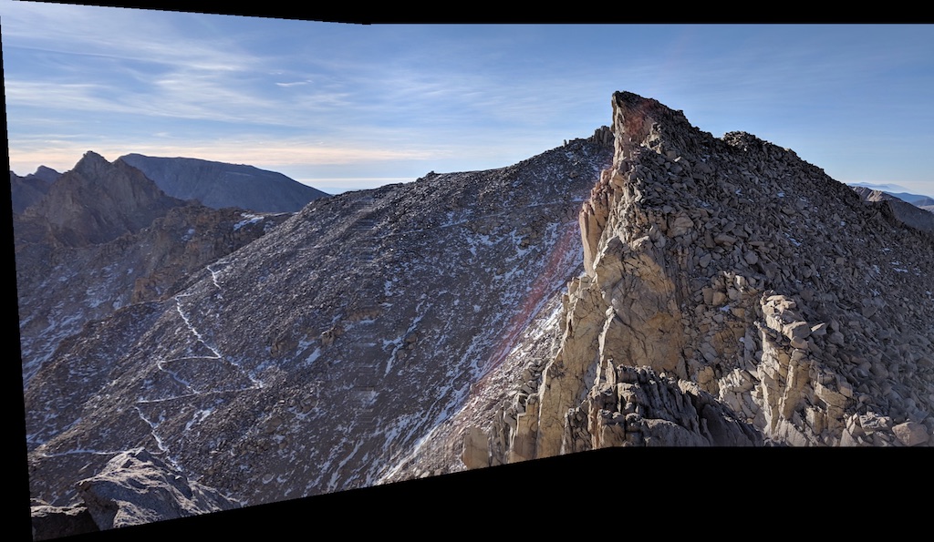
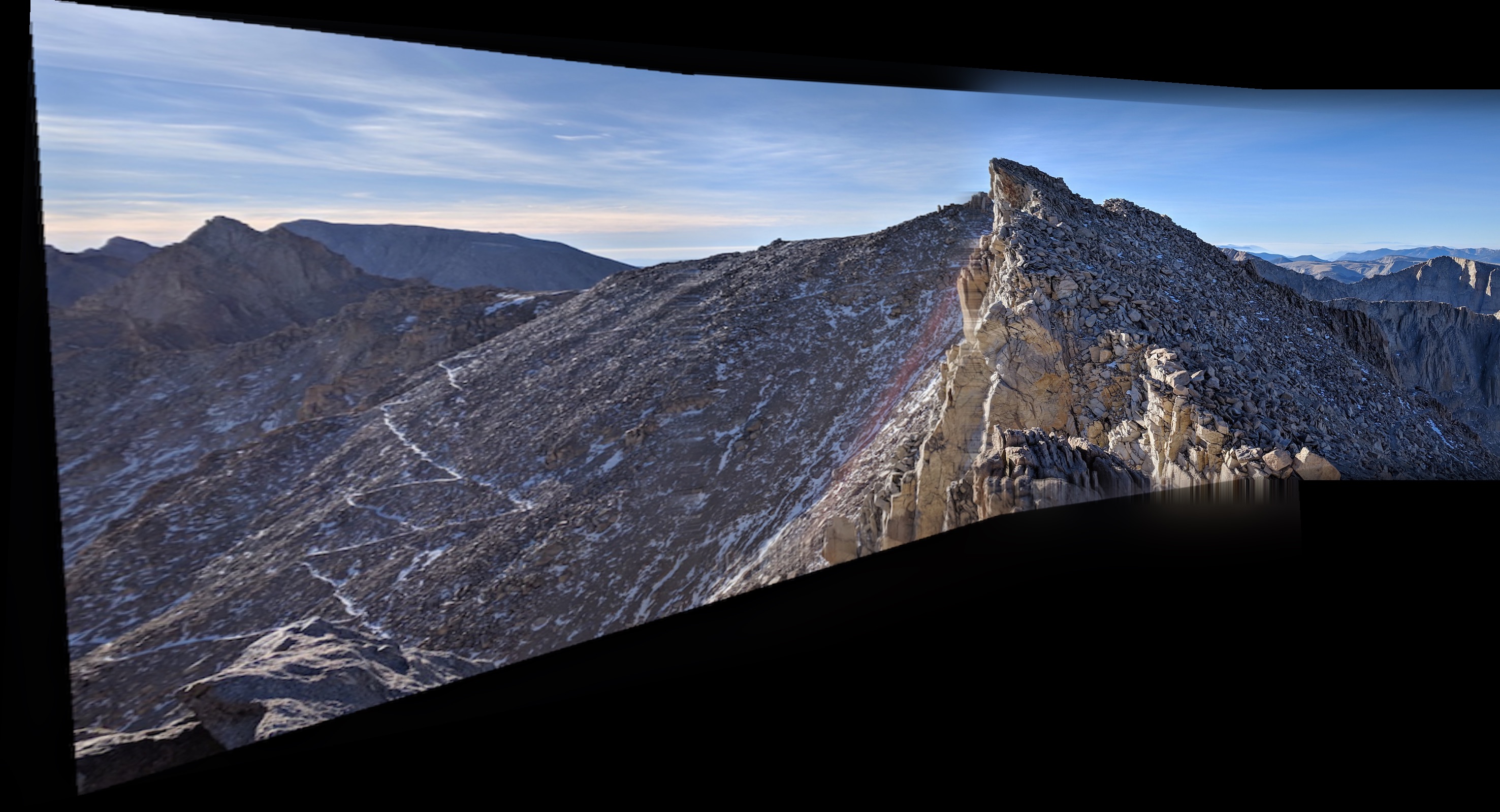
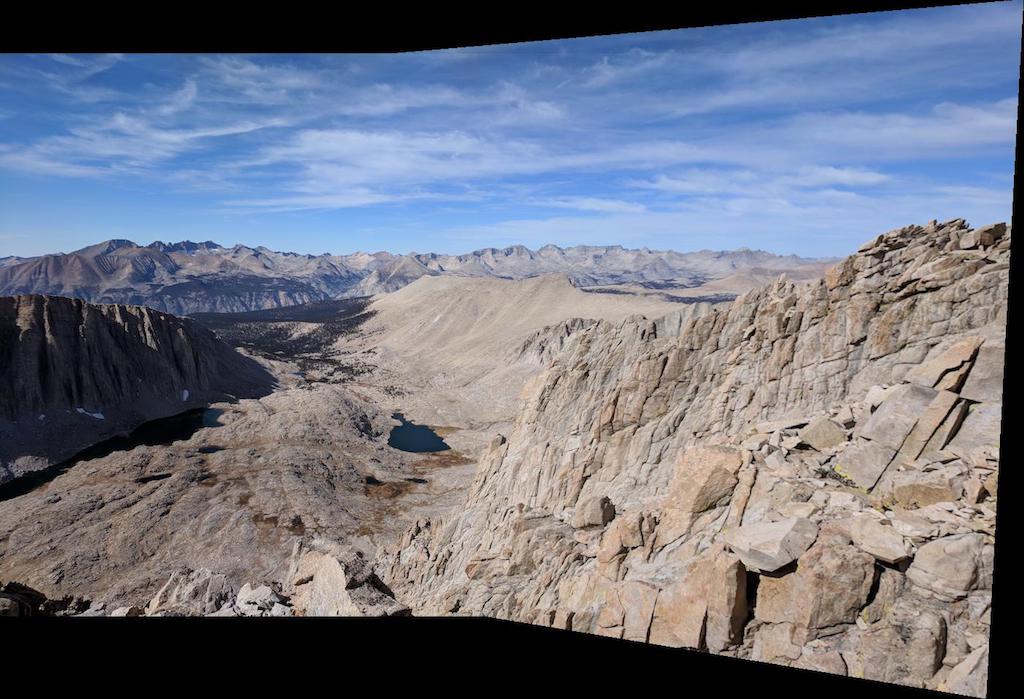
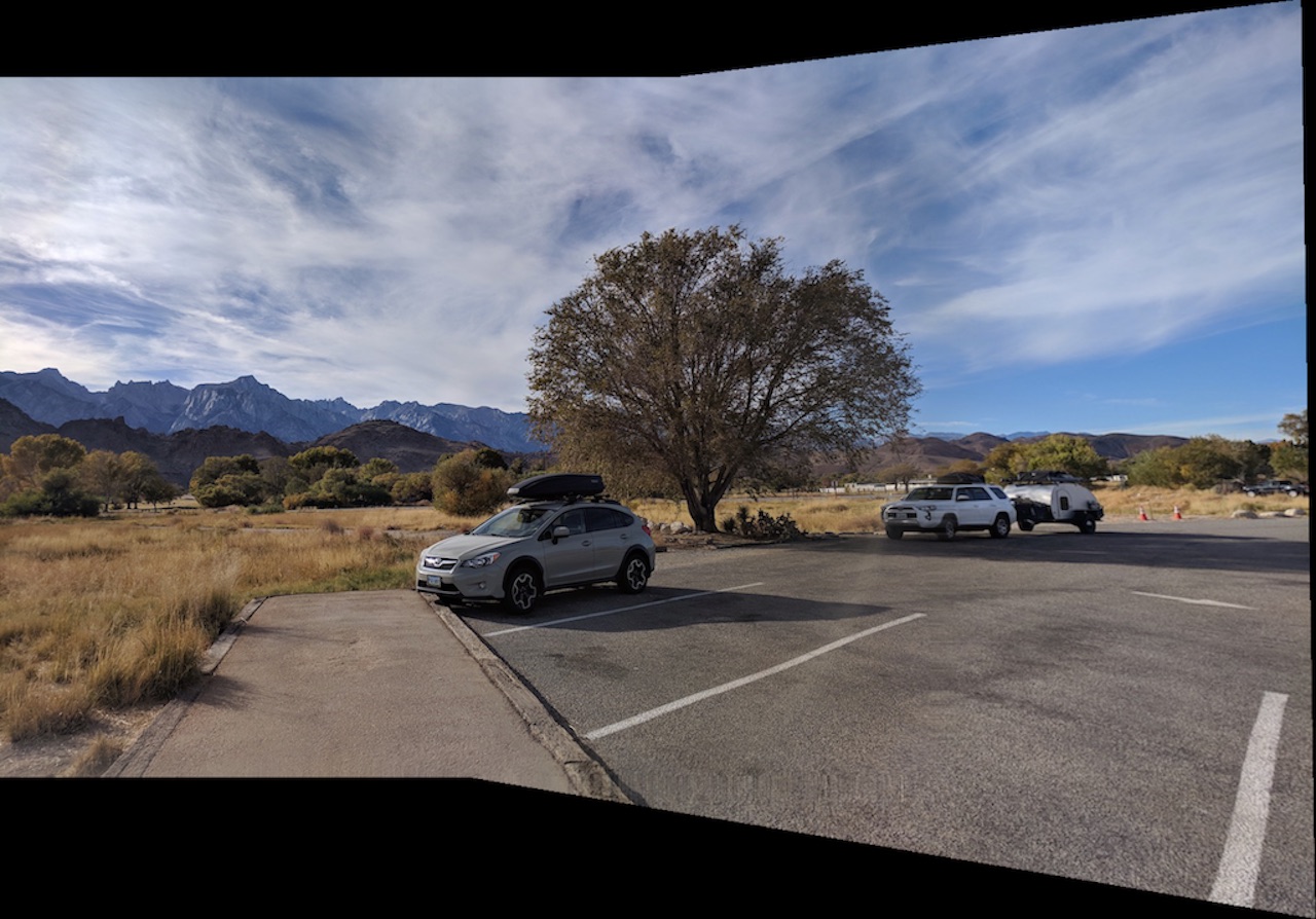
Now that we know how to warp the images we can create a mosaic! First we start with 2 images: 1 of which we warp to the plane of the other. To do this we select correspondence points between the two images and use these to generate a homography that rectifies one image to the plane of the other. We then compute the size of the target image for the panorama/mosaic and place the warped and unwarped image on their own copies of a blank background of the target image size. Since we have warped one image to the plane of the other allignment is simply a translation that we can compute using information that we found while computing our transform. We then do the correct translations to allign the images properly and use blending to properly blend the overlap.
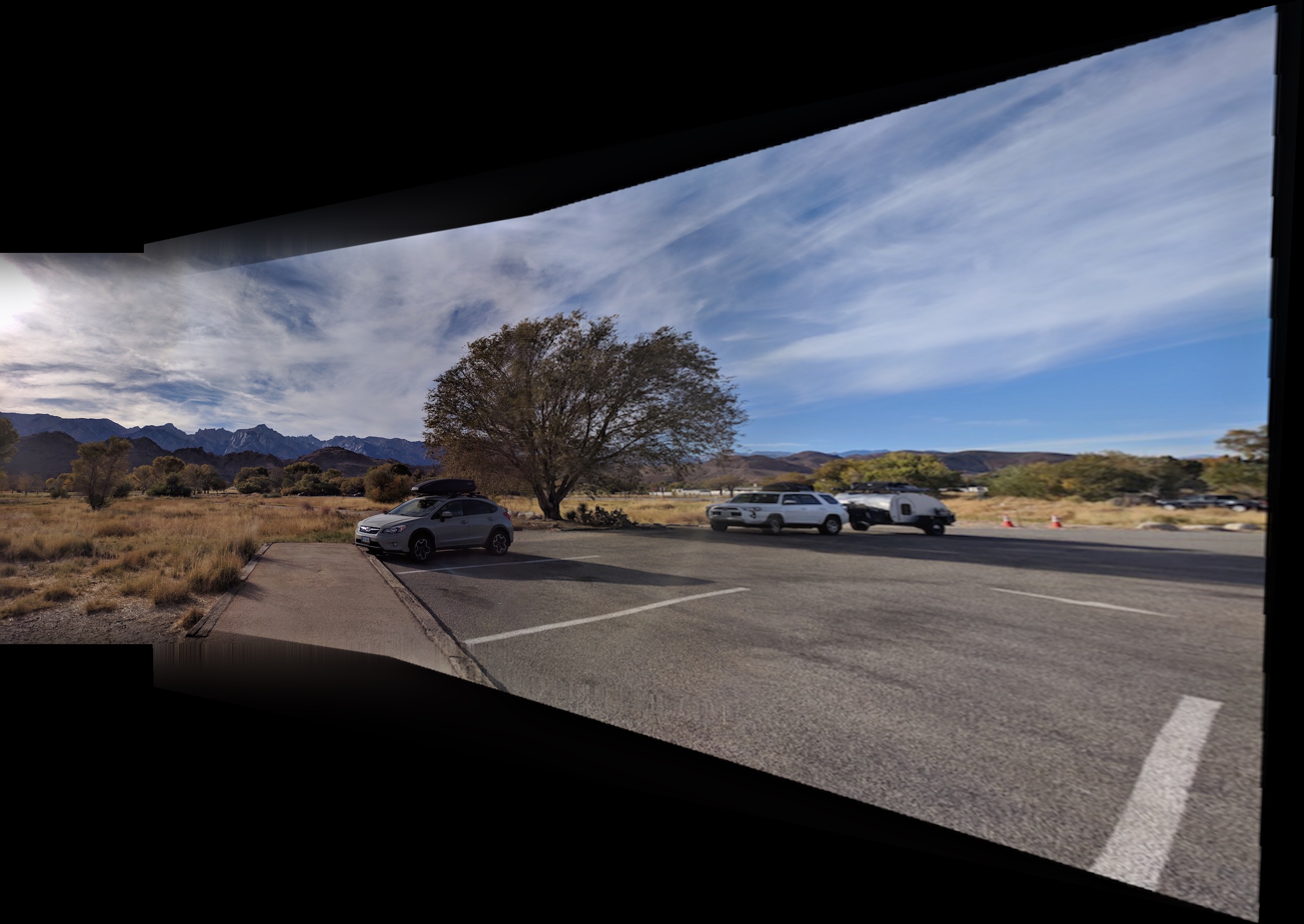
For the blending I tried two techniques: linear or alpha blending and laplacian blending. For linear blending in the overlapping region I weighted pixels from the two images with an alpha and 1-alpha respectively. These were determined by the distance of the pixel from the central point of the two images and the amount that a pixel from an image contributed was inversely proportional to its distance from it's image's center. Though this worked in a lot of images there were some visual artifacts that were apparent as seen below.
|
|
|
|
|
|
Since linearing blending was giving a lot of artifacting I switched to laplacian blending from project 3 in order to blend the two images together which gave a significantly less noticeable seam. Here is an example of laplacian blending on the same images shown above with linear blending:
|
|
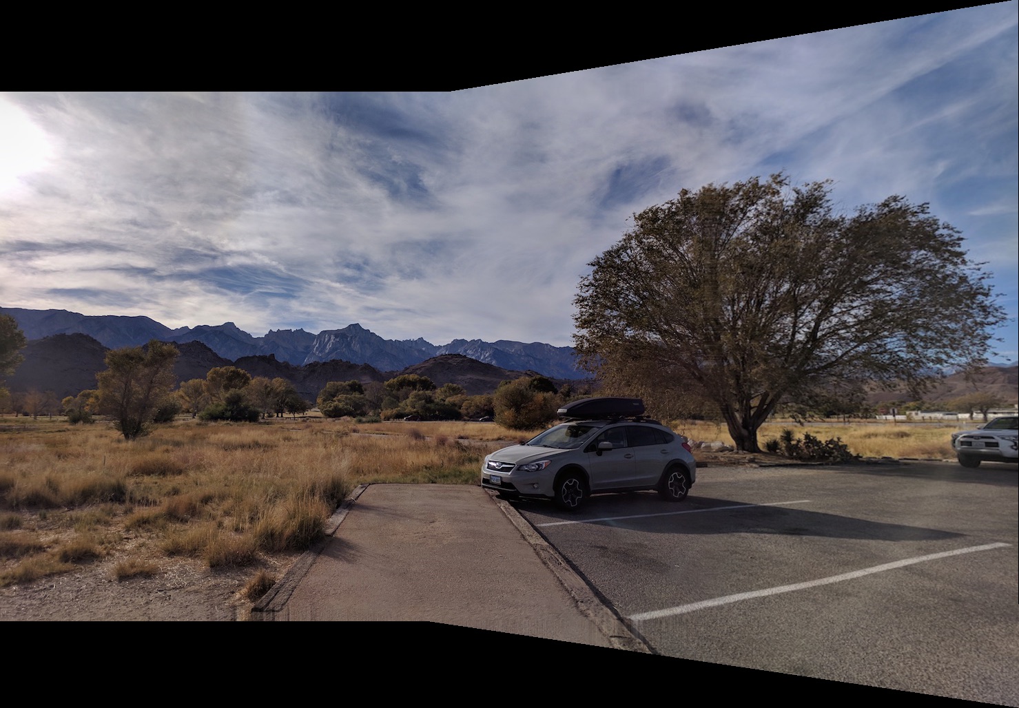
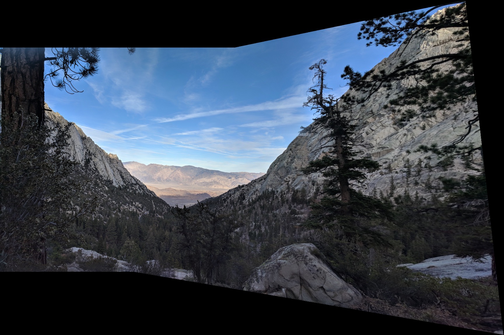
To compute panoramas with multiple images we do it in steps. We first stitch two images together and then use the result and stitch another image on that using the procedure described above. Here are some more examples of panoramas made:
|
|
|
|
|
|
|
|
|
|
|
|
|
|
|
|
|
|
|
|
I learned how to create panoramas! I also learned fundamentals about using linear algebra to transform images to project them onto desired spaces for both visual changes and to help solve certain problems. I also learned more about the nuances that go into selecting good points for a homography and how improperly choosing points or choosing a homography that warps the image too much can lead to some visually undesirable results
Use of Dlib inspired by: https://www.pyimagesearch.com/2017/04/03/facial-landmarks-dlib-opencv-python
Website template inspired by: https://inst.eecs.berkeley.edu/~cs194-26/fa17/upload/files/proj1/cs194-26-aab/website/