[Auto]Stitching Photo Mosaics
Table of Contents
1 Introduction
2 Image Warping and Mosaicing
This part of the project was definitely a rushed bit. It was due less than a week after it was released, so my results might not be the best.
2.1 Pictures
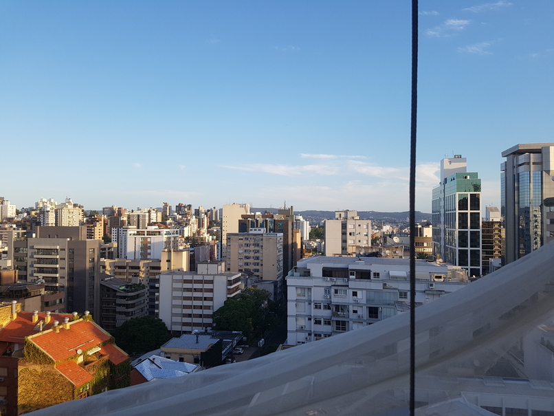
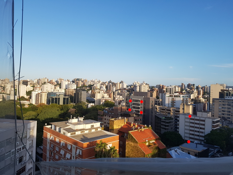
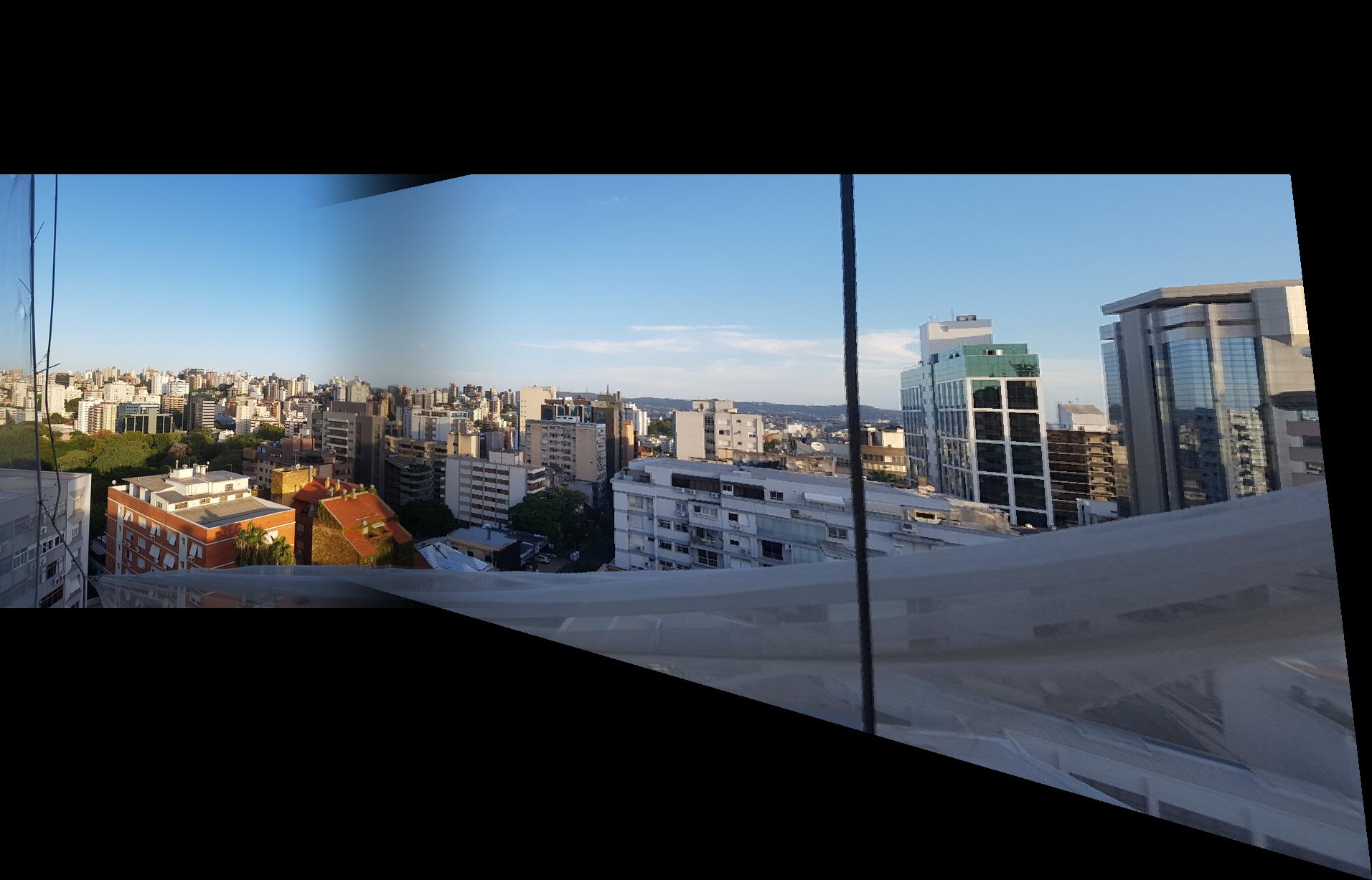
I took two pictures of the view outside my balcony in Porto Alegre, Brazil. I couldn’t do anything other than that due to the shelter in place demanded by the local government. My building’s facade is under repairs so it has a weird cloth around it that happens to be in my pictures. The photos I took are the following:

2.2 Recover Homographies
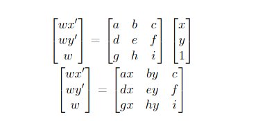
To recover the homographies, I had to do the following math reasonings:
We have that the equation given in lecture can be transformed in 2 equations
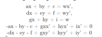
These equations can be turned into a linear system that can be used for given N points. We also know that i = 1.
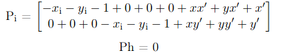
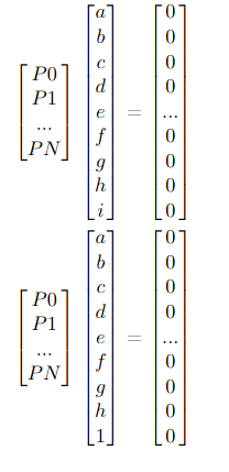
To express this constraint, we can simply add the last coefficient value to the results.
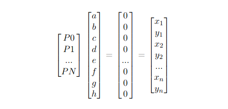
To solve this in python, we can call numpy.lstsq, which approximates the overdetermined system using the least square method.
2.3 Warp the Images
After discovering the homographies, we need to apply the transformation matrix \(H\) to all the pixels. In my method, I got a coordinate matrix from skimage.draw.polygon that refers to a rectangle and multiplied it by the inverse of \(H\) in order to inverse warp the transformation. Once having the new points, I divide them by their remaining \(w\) and colored the new “Canvas”.
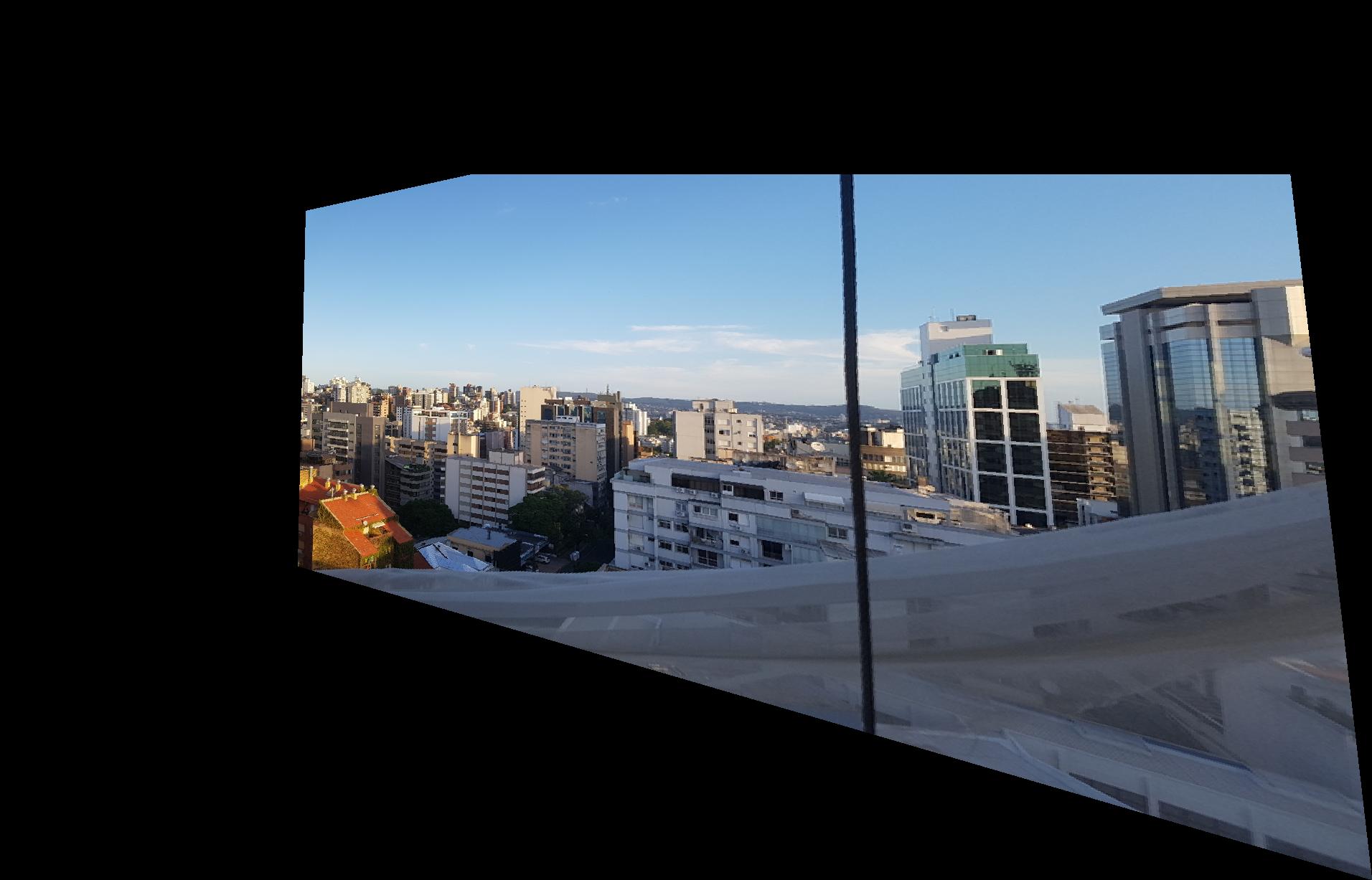
2.4 Image Rectification
Once we warped the image, we would have a rectified picture. For the final blend, I used this geometry:

Now, applying the transformation to the image on the right, we get the following result:
2.5 Mosaic Blending
Having the warpped image, it’s time to blend them together! We do so by generating a canvas large enough to contain both images. Since both will be mapped in the same proposed space (pixels of correspondence in the same place), the blending ends up being more of an alpha calibration blending. To do the calibration, I used a cosine function powered to a given exponent. I also decided to start blending after we had reached the middle of the image, which I realize that wouldn’t work if we had more than 50% of overlapping. Also, I only set my program to blend in the left to right direction. The alpha blending equation results are the following given an exponent:
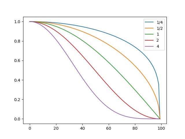
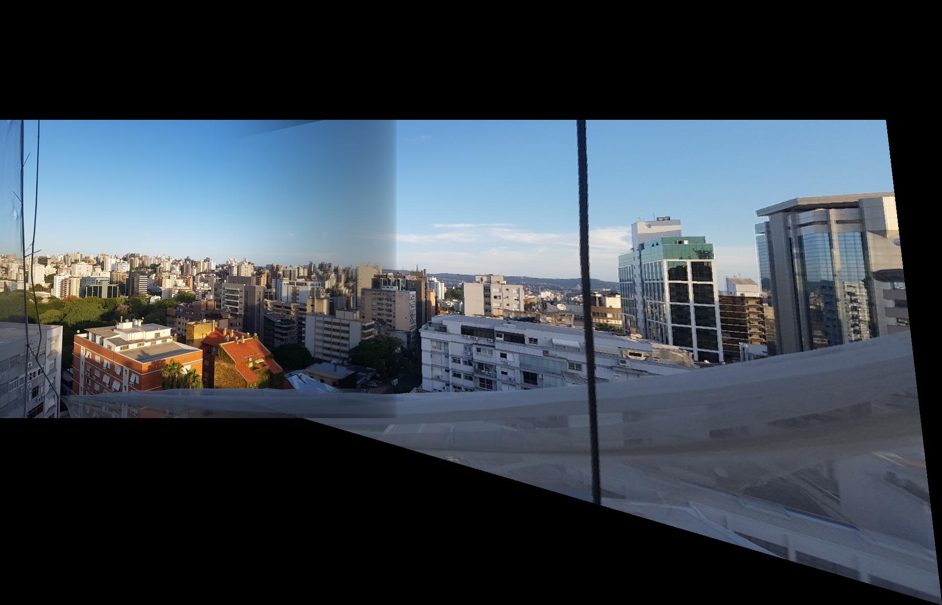
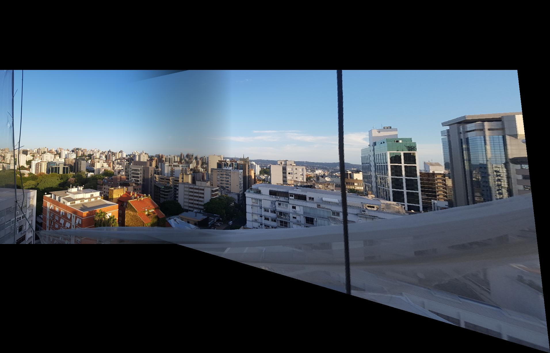
These were the results:
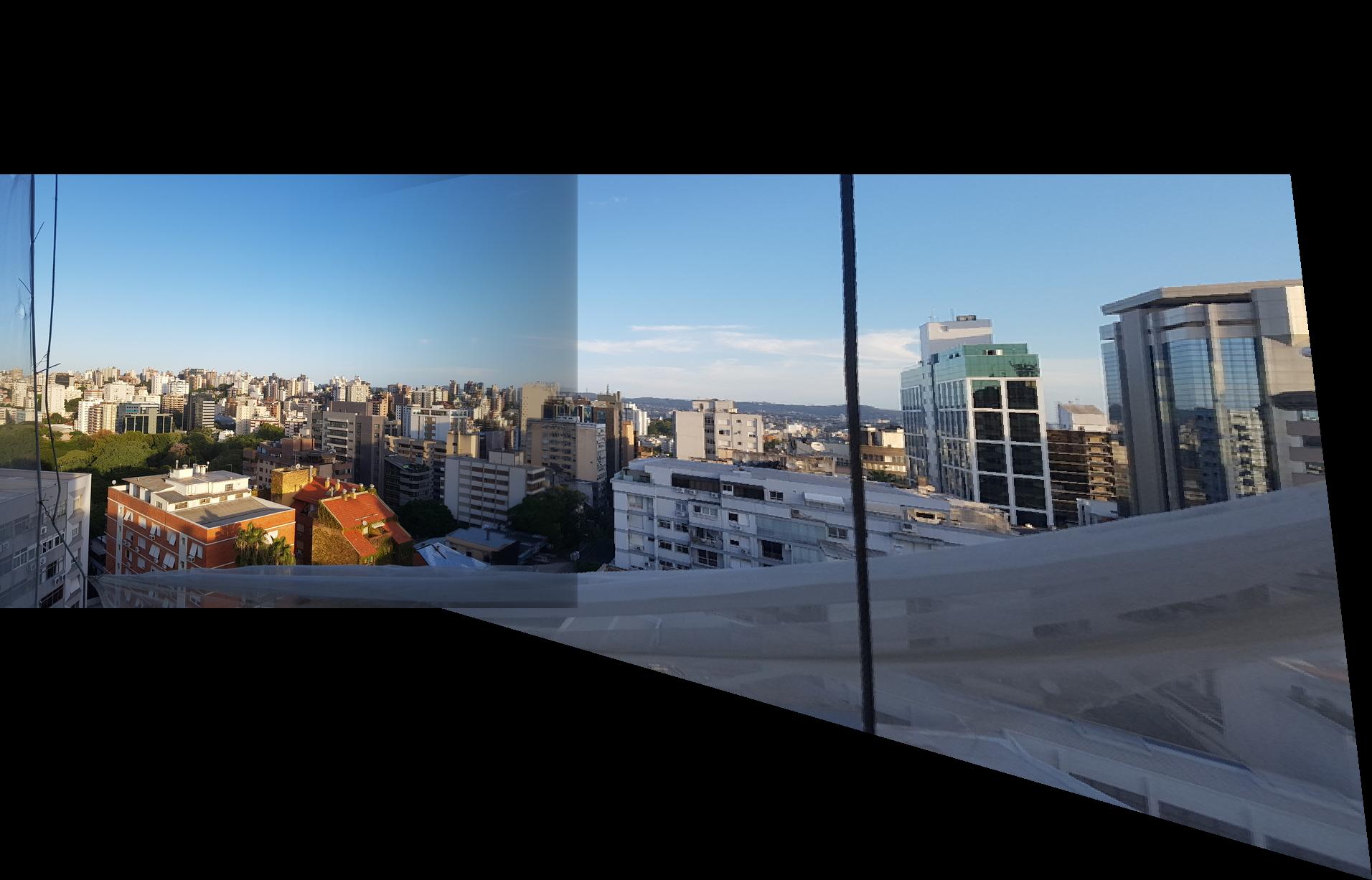
exponent \(\frac{1}{4}\) on the left and \(\frac{1}{2}\) on the right.
exponent \(1\).

exponent \(2\) on the left and \(4\) on the right.
Given these results, I decided that the exponent of \(2\) gave me the best result because it blended well without losing too much of the first image.