Project 6: [Auto]Stitching Photo Mosaics¶

Author:	Tianrui Guo <aab>

Project Spec: https://inst.eecs.berkeley.edu/~cs194-26/fa18/hw/proj6/

Part A: IMAGE WARPING and MOSAICING¶

Project Overview¶

The goal of this project is to warp images to create image mosaics.

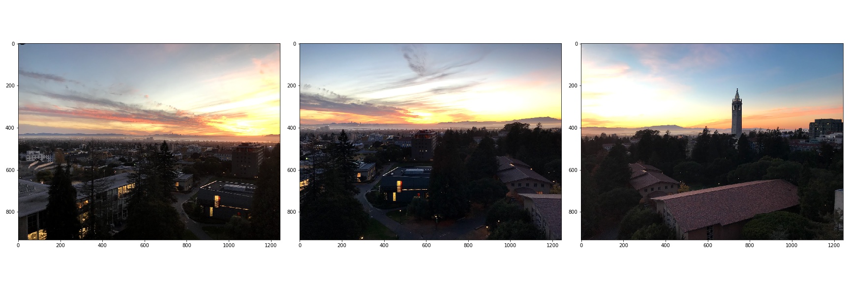
Shoot the Pictures¶

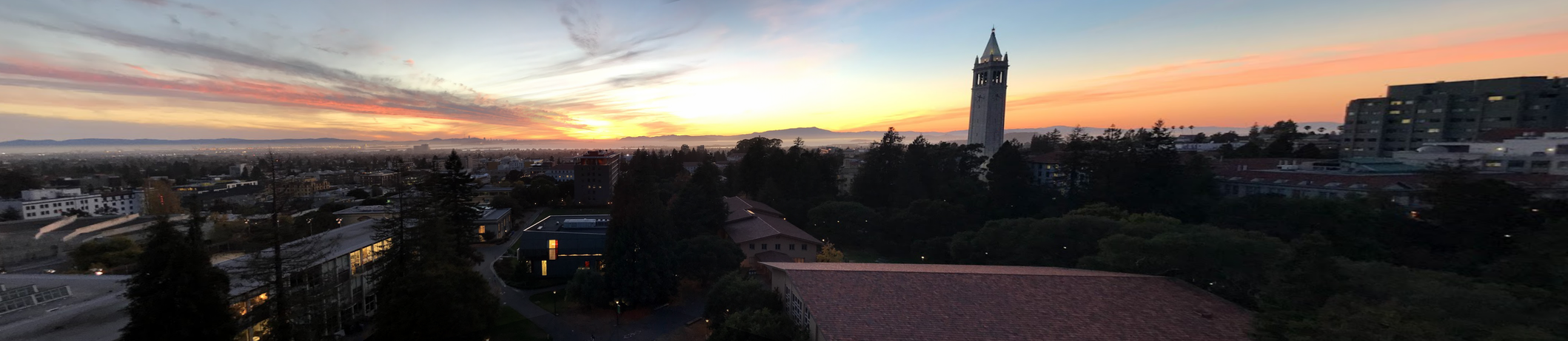
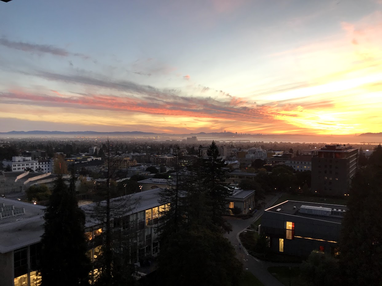
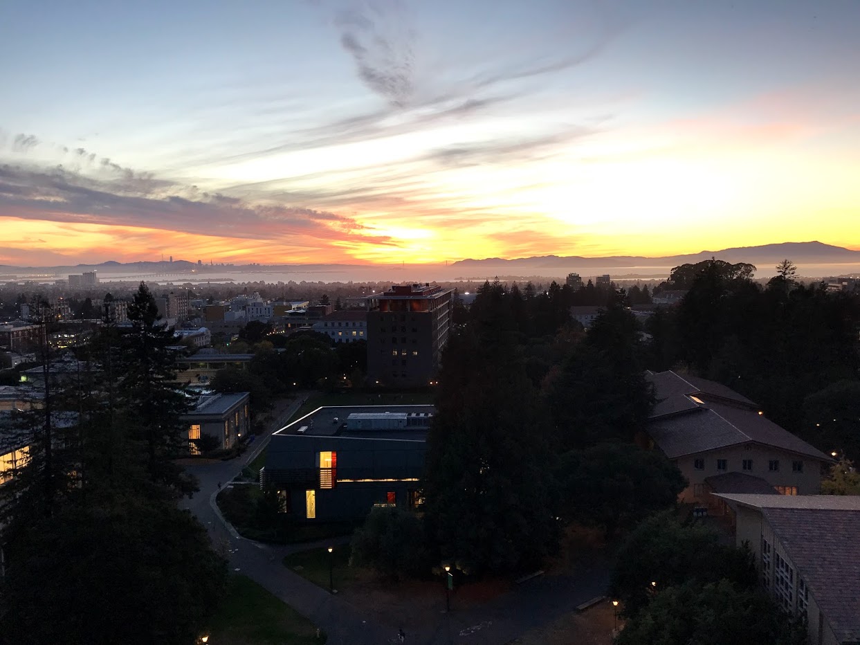
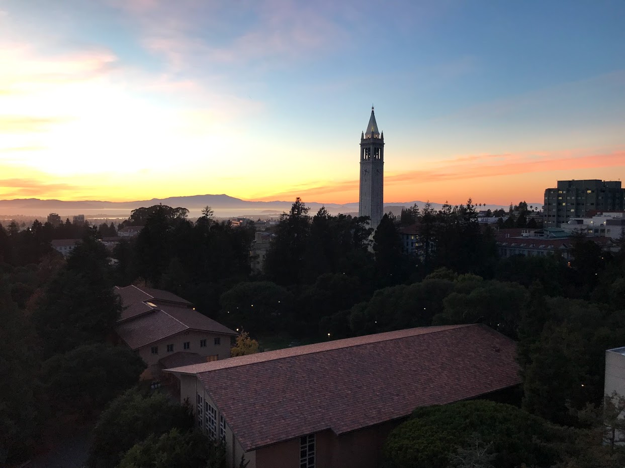
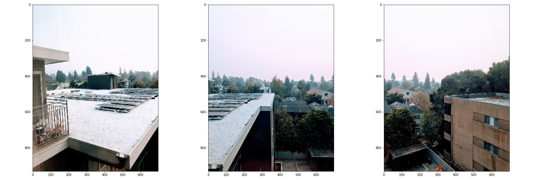
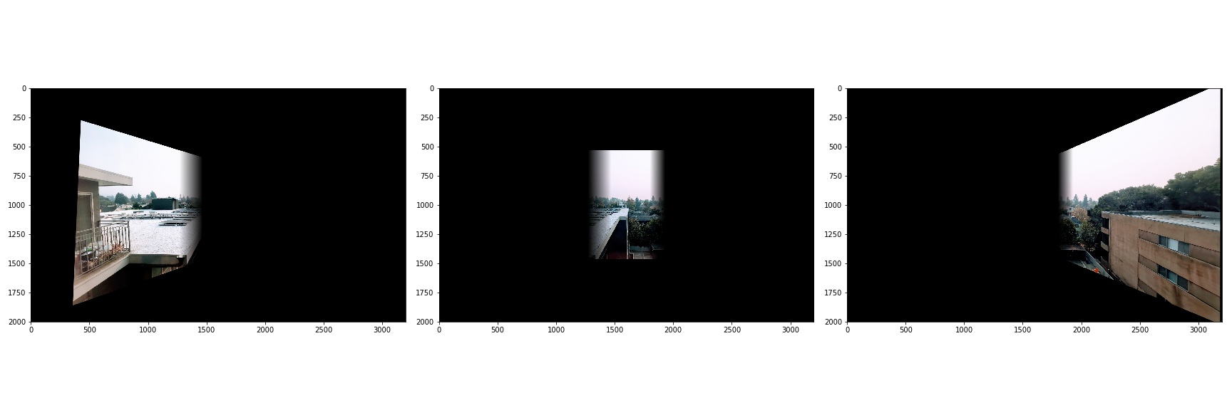
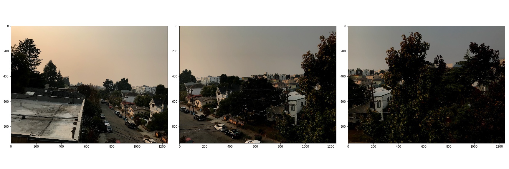
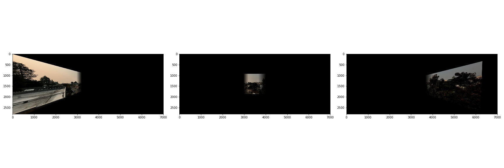
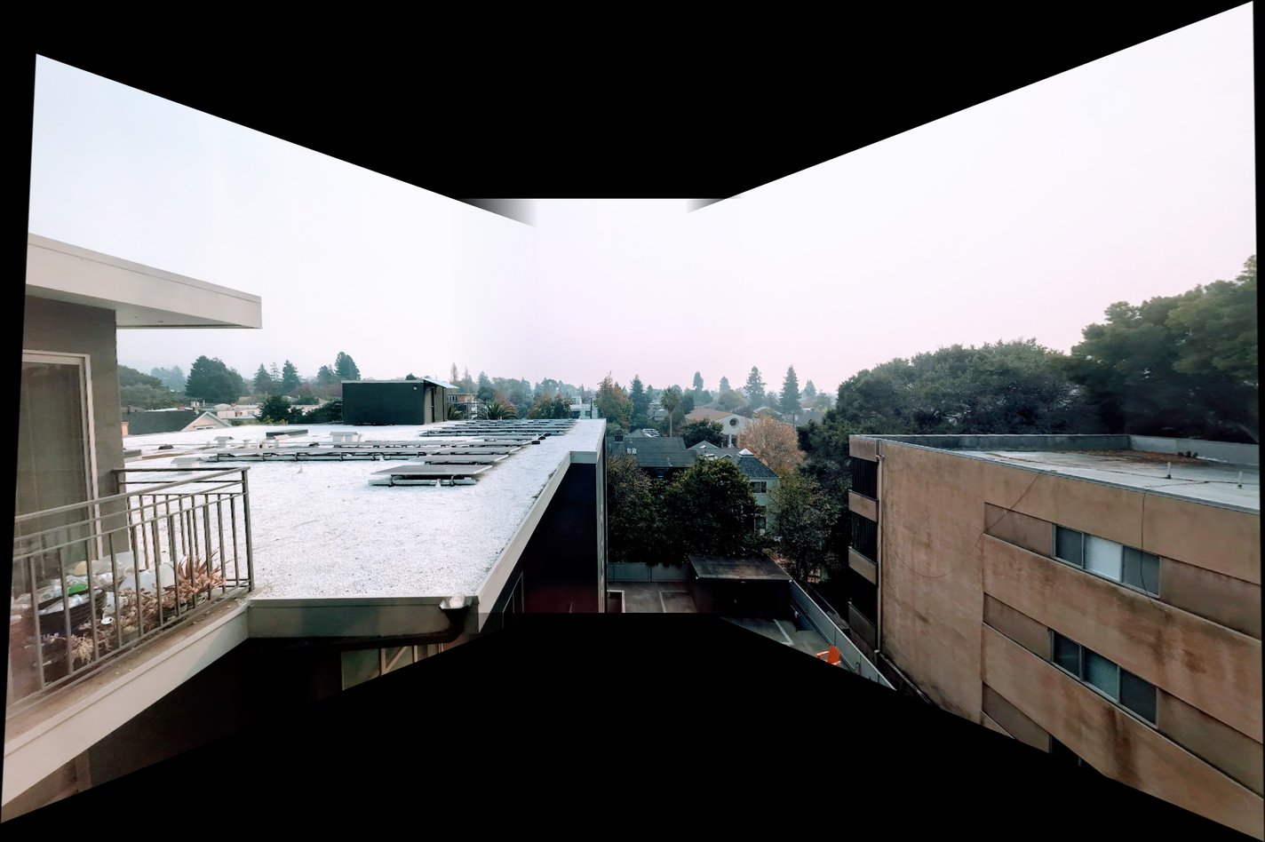
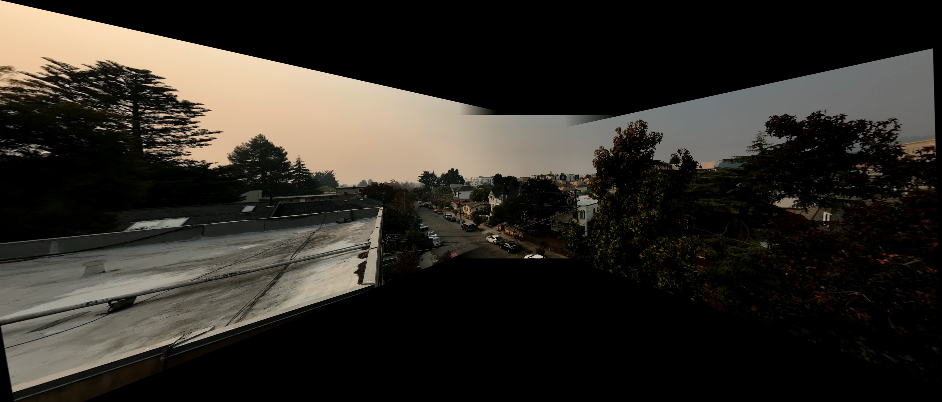
This first part of this project involved taking some pictures. When taking multiple photographs to merge together for an image mosaic, it is important to lock the focal length and exposure, and to ensure that the axis of rotation goes through the camera lens. Here is one sequence of photographs that I took:

Recover Homographies¶

The next part of the project is to label point correspondences in the images and compute the transformation between two sets of corresponding points. To select point correspondences, I used Matlab’s cpselect tool, and I tried to select points that correspond to corners for better accuracy.

Once we have these point correspondences, the next thing to do is to find the transformation between points in two images. The transformation in this case is a homography, and the equation that describes the transformation is:

\[\begin{split}\begin{align} p' &= H p\\ \begin{bmatrix}wx'\\ wy'\\ w\end{bmatrix} &= \begin{bmatrix}a & b & c\\ d & e & f\\ g & h & 1\end{bmatrix} \begin{bmatrix}x\\ y\\ 1\end{bmatrix} \end{align}\end{split}\]

Where \(w\) is some unknown value for each pair of points and \(H\) is the matrix that we are trying to solve for. Expanding out the multiplication, we get:

\[\begin{split}\begin{align} wx' &= ax + by + c\\ wy' &= dx + ey + f\\ w &= gx + hy + 1 \end{align}\end{split}\]

We can see that if we multiply the last equation by \(x'\) or \(y'\), we can substitute the right hand side into the top two equations to eliminate \(w\). Thus, we now have a system of linear equations of the form:

\[\begin{split}\begin{align} 0 &= ax + by + c - gxx' - hyx' - x'\\ 0 &= dx + ey + f - gxy' - hyy' - y'\\ \end{align}\end{split}\]

Since there are 8 unknown values and each pair of points yields two new equations, we need 4 pairs of points to recover the homography. However, in this project, I chose between 16 and 24 pairs of points for each pair of images, and then found the least squares estimate for the values of \(H\). This helps to reduce the effects of imprecise point picking.

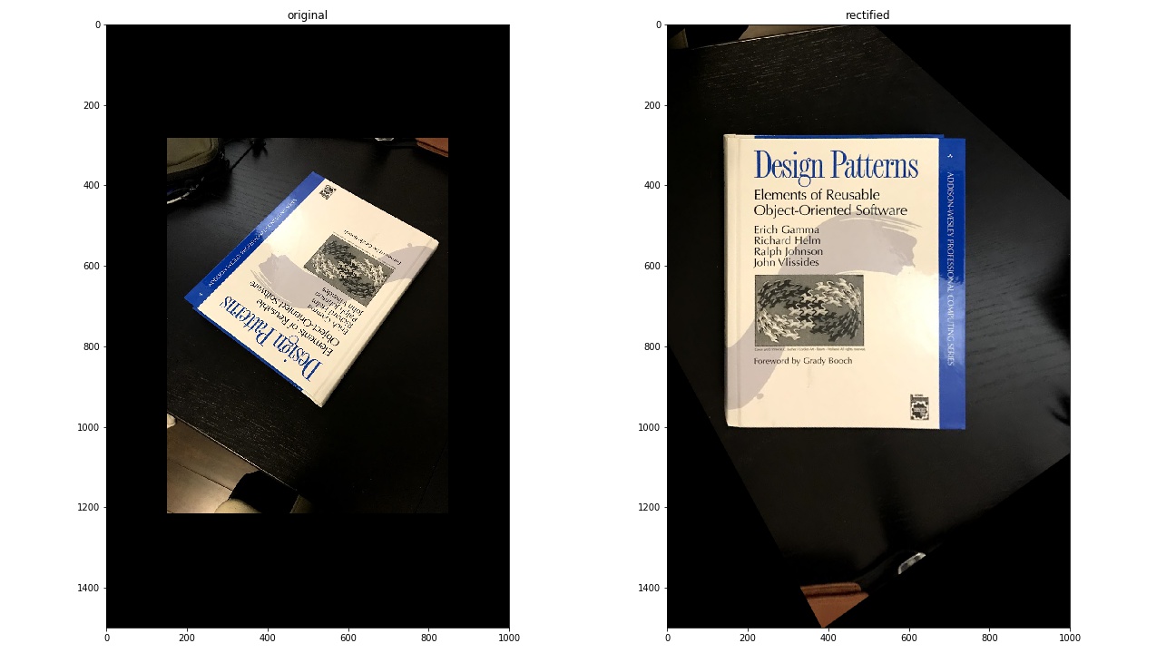
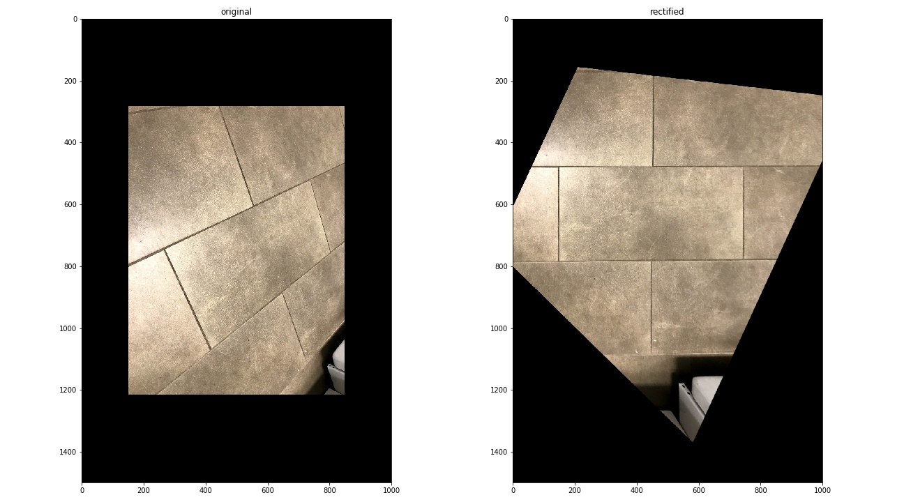
Image Rectification¶

Now that we have a function to compute homographies, we can use that to rectify images. The idea here is that we can take a picture of something rectangular at an off angle, select the corners of the rectangle, and then compute a homography that maps those corners into a rectangle. Here are the results:

Book¶

Tiles¶

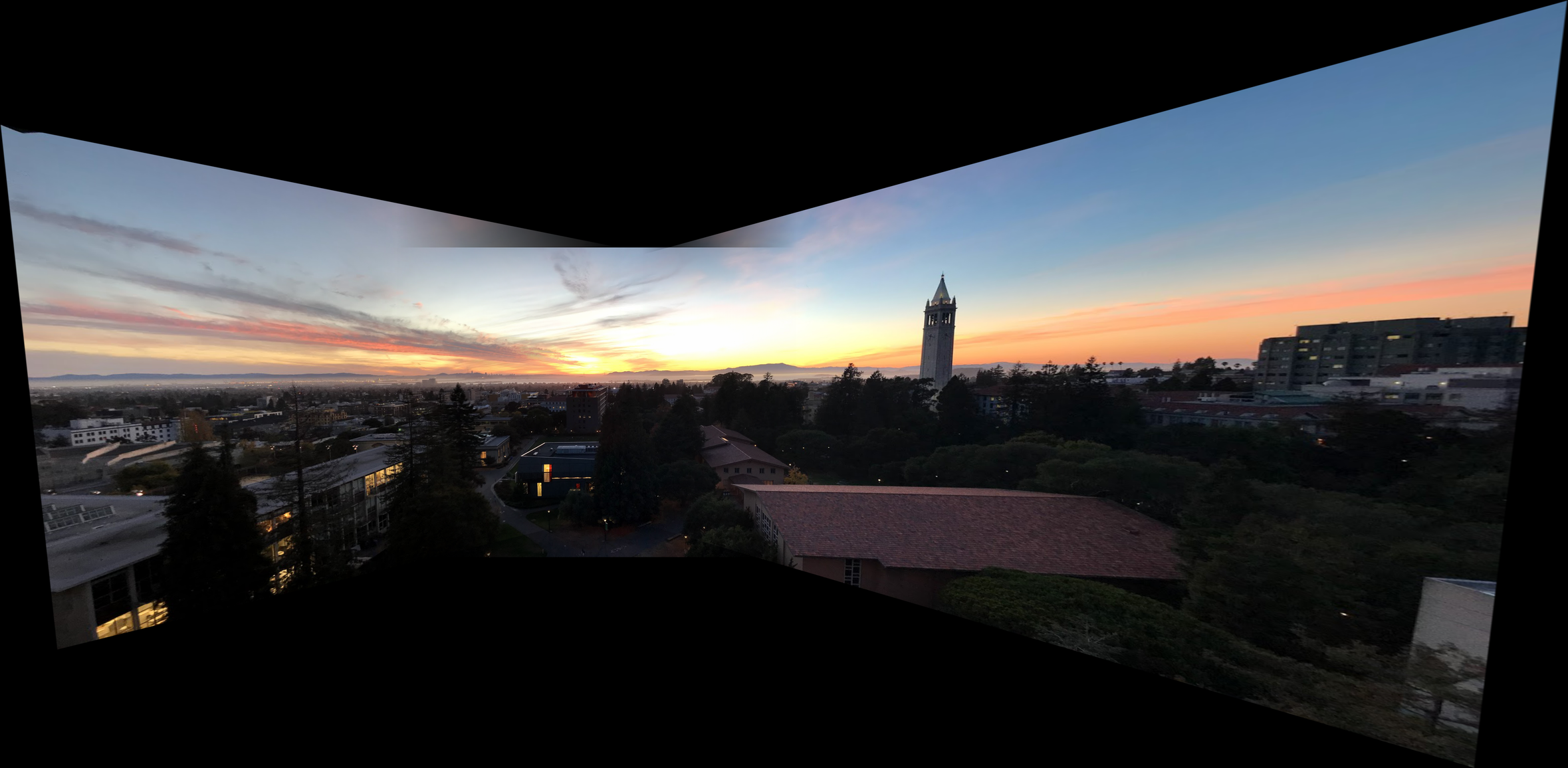
Blend the Images into a Mosaic¶

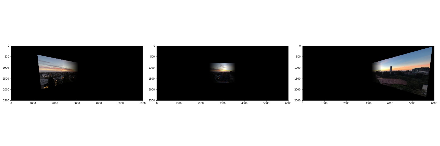
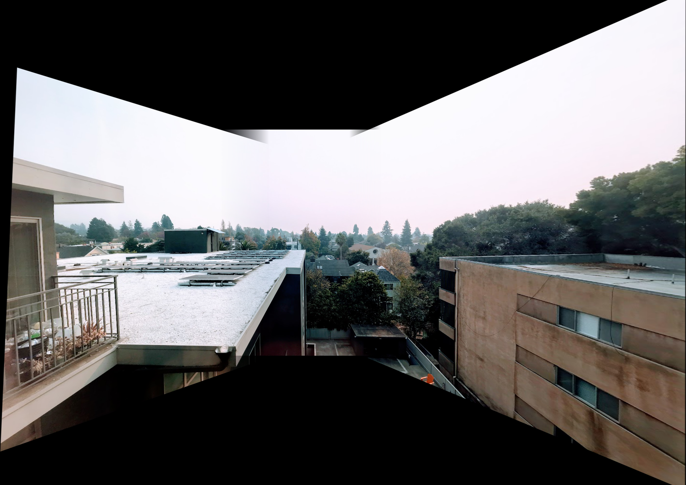
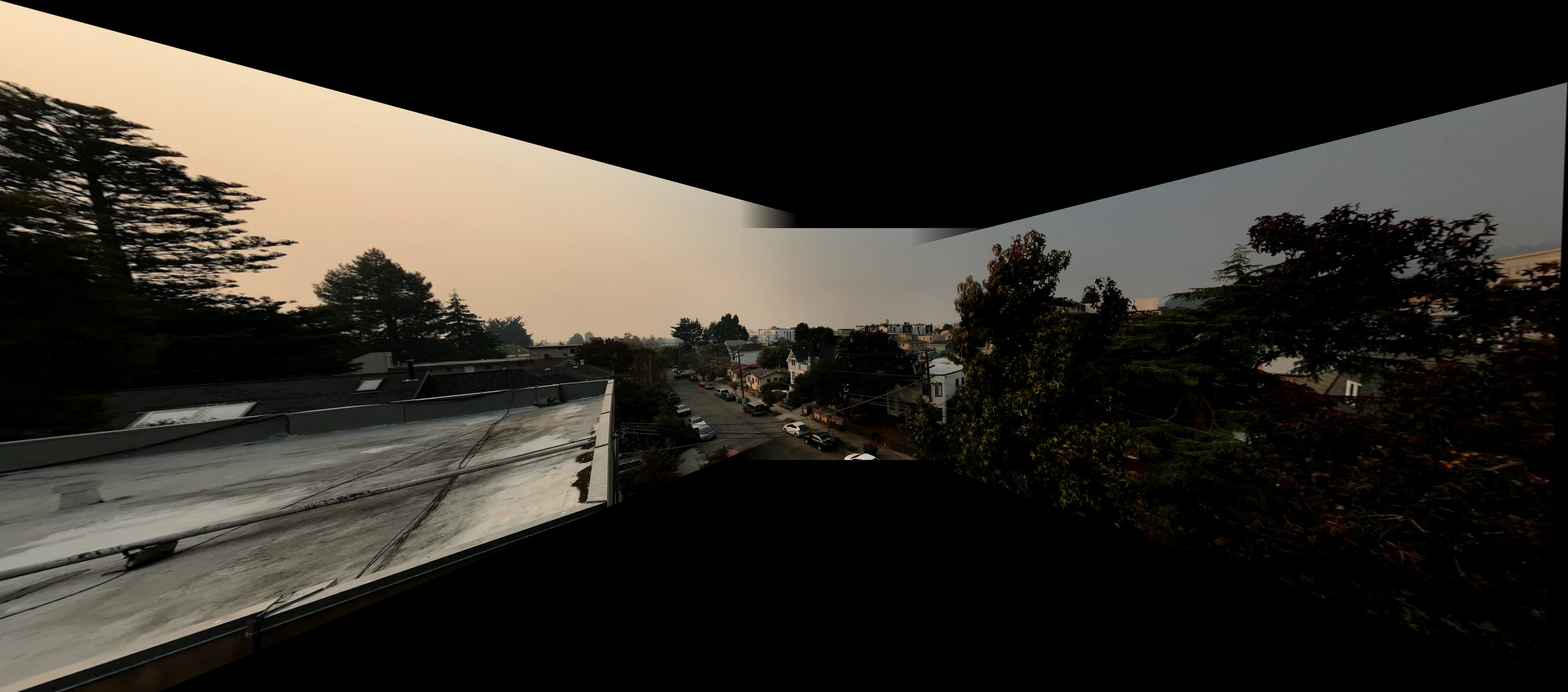
With the code from the previous parts, we are almost ready to produce mosaics. The only thing left to do is to blend the morphed images together to hide the transitions between images. To accomplish this, we used simple alpha blending. Here are the results:

Berkeley Campus¶

Cropped (By hand)¶

Original Images¶

Warp + Alpha Mask¶

Berkeley Buildings¶

Cropped (By hand)¶

Original Images¶

Warp + Alpha Mask¶

Berkeley Street¶

Cropped (By hand)¶

Original Images¶

Warp + Alpha Mask¶

Lessons Learned¶

In this project, I learned about how to morph images to create mosaics. I learned how to compute a homography from a set of point correspondences, how to use that homography to warp an image, and also how to blend warped images together.

Part B: FEATURE MATCHING for AUTOSTITCHING¶

Project Overview¶

The goal of this project is to automatically generate a set of point correspondences for mosaic stitching.

Step 1: Detecting Corners¶

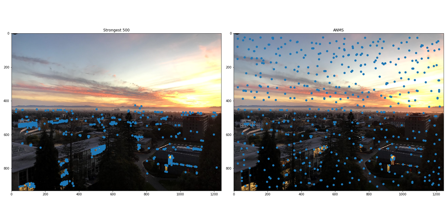
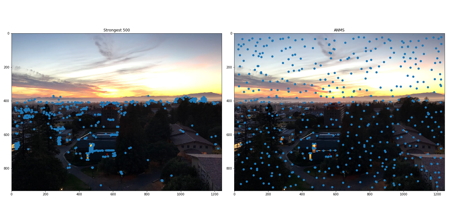
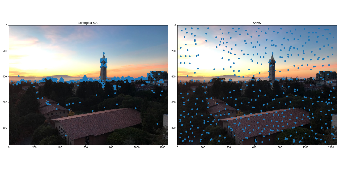
In the first part of the project, we detect the corners in an image using Harris Detector. To ensure that the corners are spatially spread out in the images, we use the Adaptive Non-Maximal Suppression algorithm. In this algorithm, we iterate through each point returned by the Harris Detector, and compute its radius. This value is the distance to the closest point with a corner strength that is 10 percent greater than its own value. The points we select will be the subset of points with the largest radii.

Results¶

Here are some results comparing simply taking the largest corner strengths to using the ANMS algorithm:

Step 2: Feature Descriptor¶

Now that we have a set of interest points, the next thing to do is to compute feature descriptors from each interest point. These feature descriptors will be axis aligned 8x8 patches that are downsampled from 40x40 windows centered on interest points. One important thing to do for this step is to subtract out the mean and normalize to unit variance. We will use these feature descriptors to match points across images.

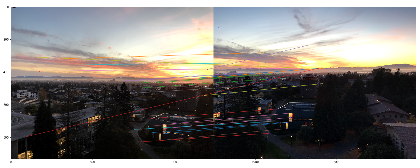
Step 3: Feature Matching¶

To match interest points across images, we compute the pairwise distances (L2 norm) of the feature descriptors. If we have a point \(p_1\) on one image a a point \(p_2\) on the other image, accept the two points as a pair if

\[||d(p_1) - d(p_2)||_2 < 0.6 ||d(p_1) - d(p')||_2 \forall p' \in I_2, p' \neq p_2`\]

Where \(d\) is the function that computes the feature descriptor from a point and \(I_2\) is the second image. The idea here is that the best match should be much better than the next best match when it comes to matching interest points. Otherwise, if the top two choices are similar in terms of distances, then it is much more likely that this is an inaccurate pairing.

Results¶

_images/berkeley_left_correspondences.png

_images/berkeley_right_correspondences.png

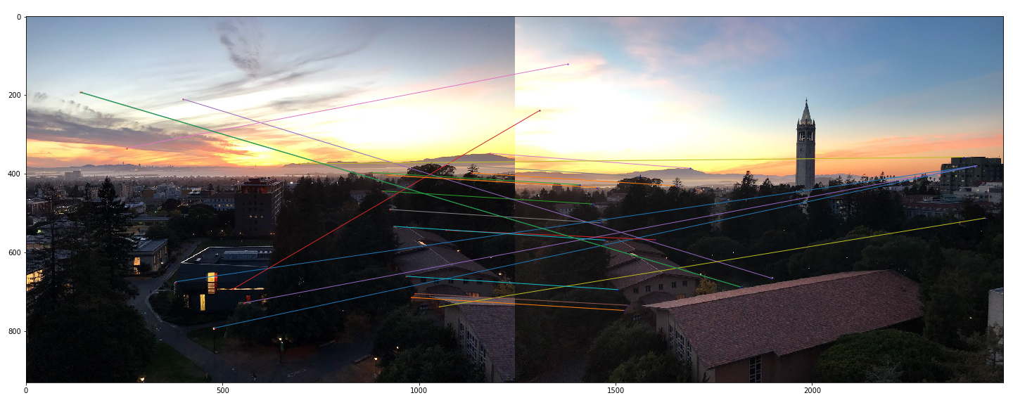
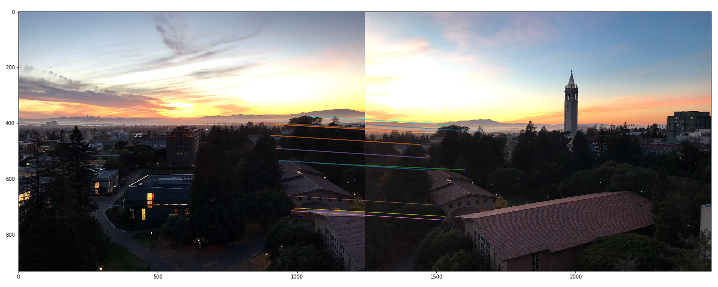
Step 4: RANSAC¶

In the above results we can see that we still have some bad pairs. The purpose of RANSAC is to compute a homography that only uses accurate pairs. The idea behind this algorithm is that we can randomly choose a set of 4 pairs to compute a homography, and then apply that homography to all of the paired up points in one image to see how many of them get accurately transformed. By repeating this with many randomly generated sets of pairs and keeping track of the largest subset of points that were accurately transformed, we can then compute the final homography using that maximal subset. The intuition as to why this algorithm should work is that pairs that were inaccurately matched will all be different in their own ways and thus would not be fit by any one homography, but all of the accurately matched points will work under the same homography.

Results¶

_images/berkeley_left_correspondences_RANSAC.png

_images/berkeley_right_correspondences_RANSAC.png

Final Results¶

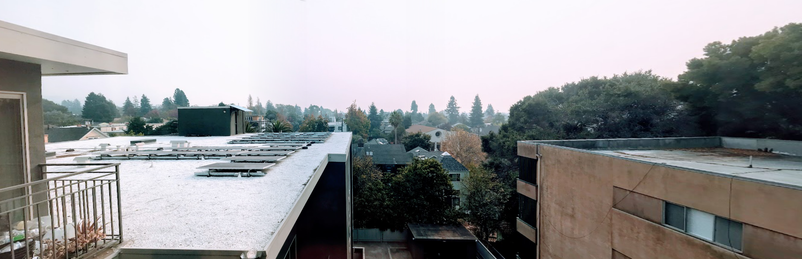
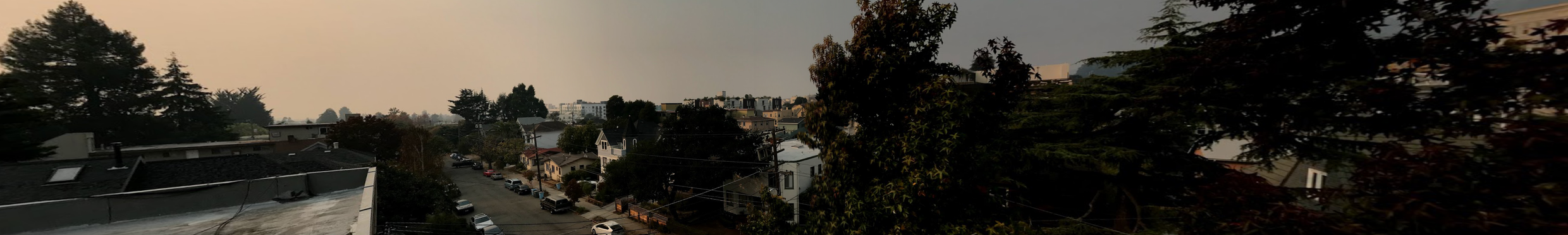
Here are panoramas generated from the same set of images as the first part, only this time we automatically align the images.

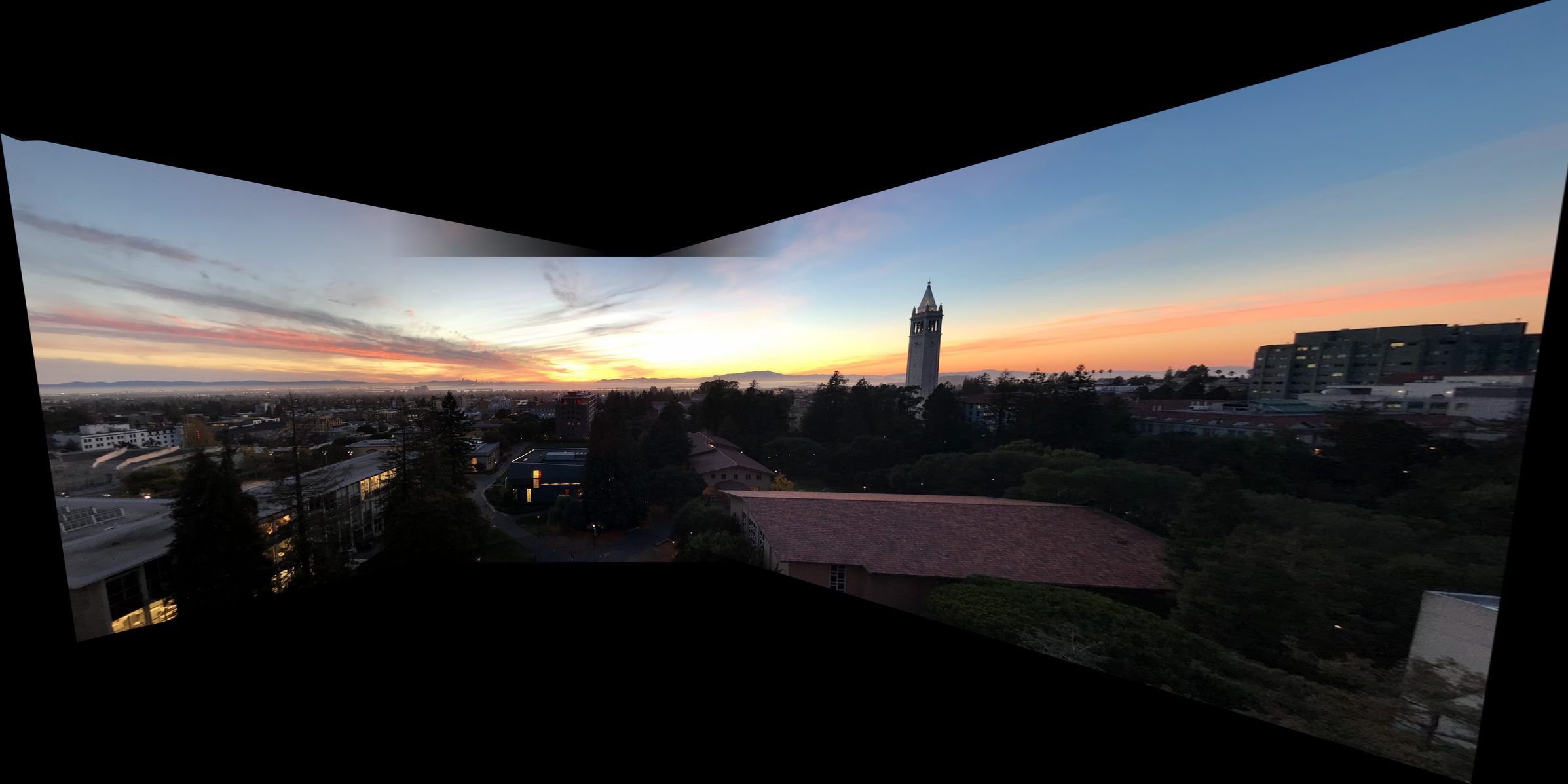
By zooming into the tree on the last panorama, we can see that the auto-stitching algorithm actually did a better job of combining the images when compared to the manually aligned image. Beyond that, there are only very subtle differences between the panoramas generated by the two different approaches. However, the auto-stitching approach involves a lot less manual work.

Reflections¶

In this part of the project, I learned how to automatically align images to create mosaics. The coolest thing I learned is this project was the RANSAC algorithm to filter out bad correspondences and compute an accurate homography.