Part A
The goal of this part is to create an image mosaic by doing projective warping, resampling and composing the images together.
Image Rectification
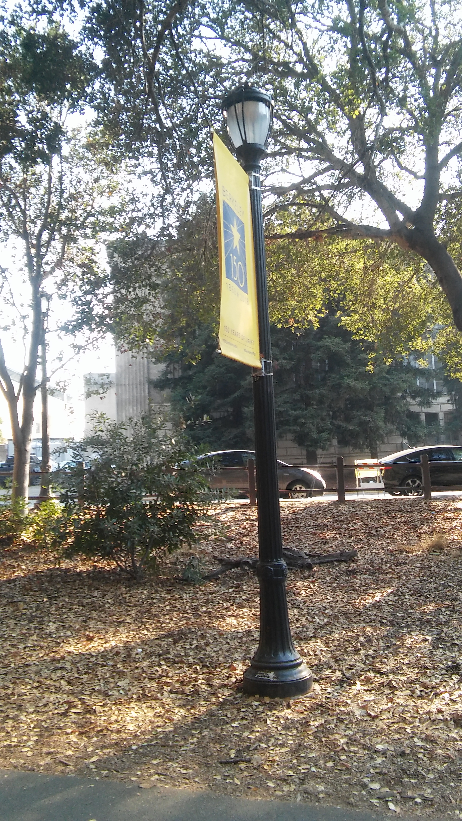
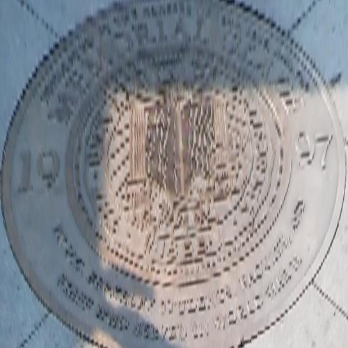
In order to test that the homography and inverse warping work correctly, we will take a few sample images with planar surfaces and warp them to get a frontal-parallel plane. The first example is a picture of a Berkeley 150 poster. Here is the picture.
Berkeley 150 Poster
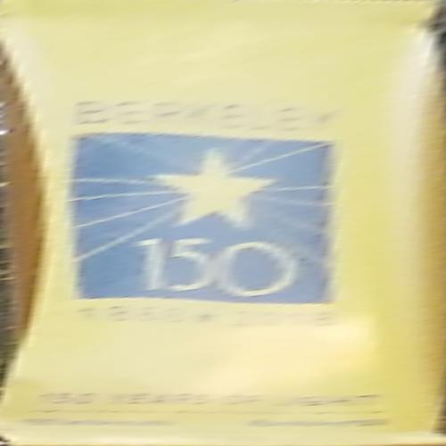
Rectifiied Berkeley 150 Poster
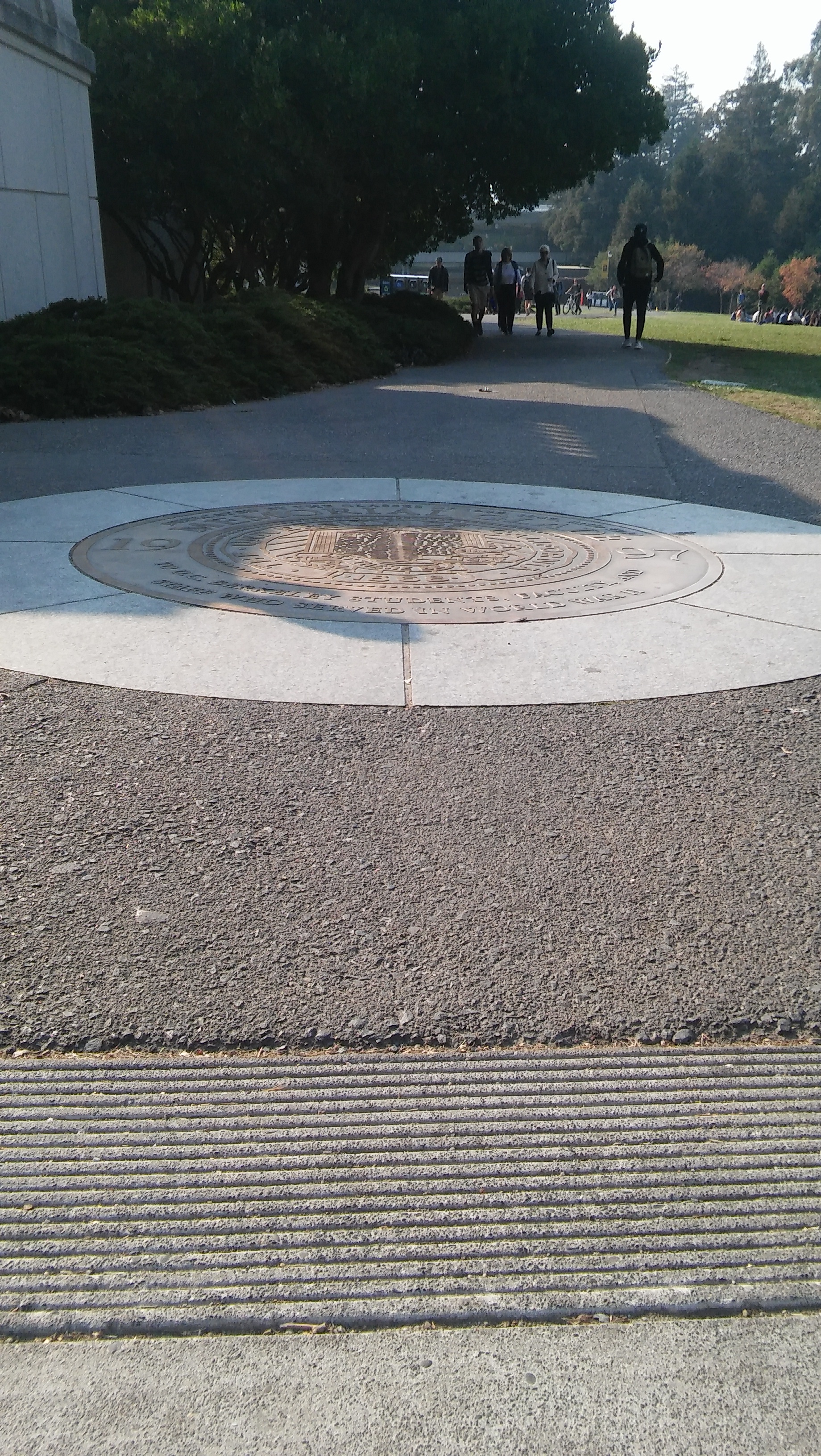
Cal Seal and the rectifiied image
Blend the images into a mosaic
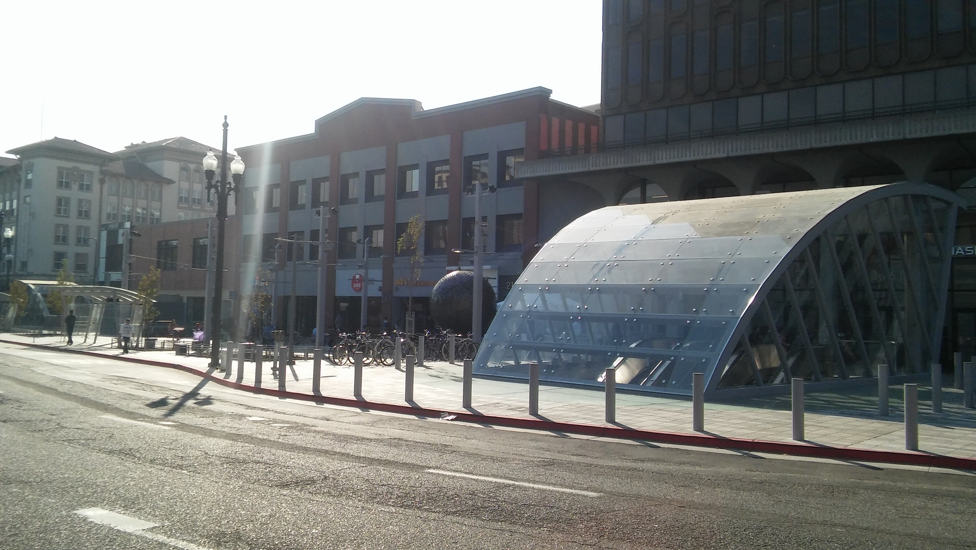
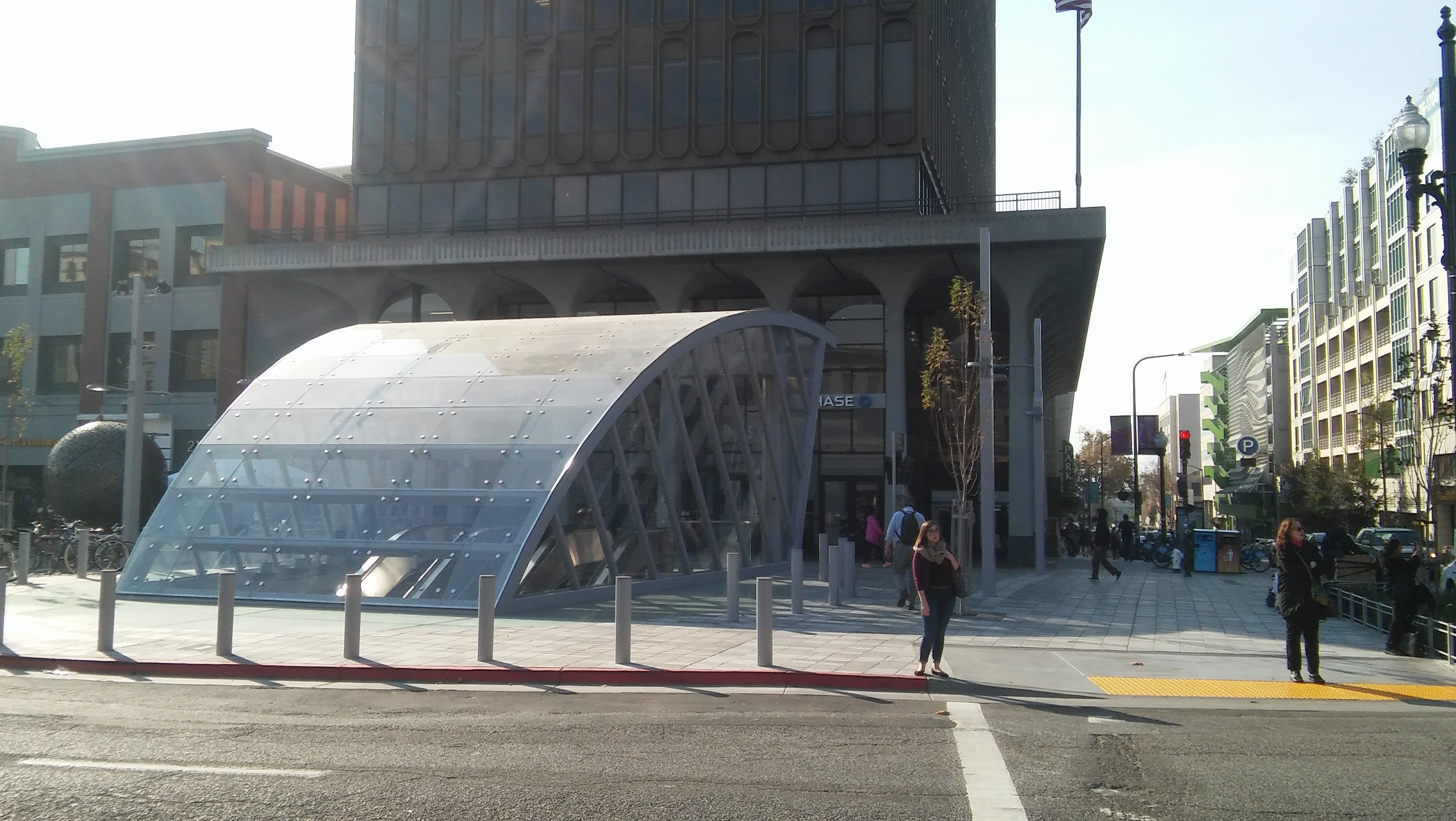
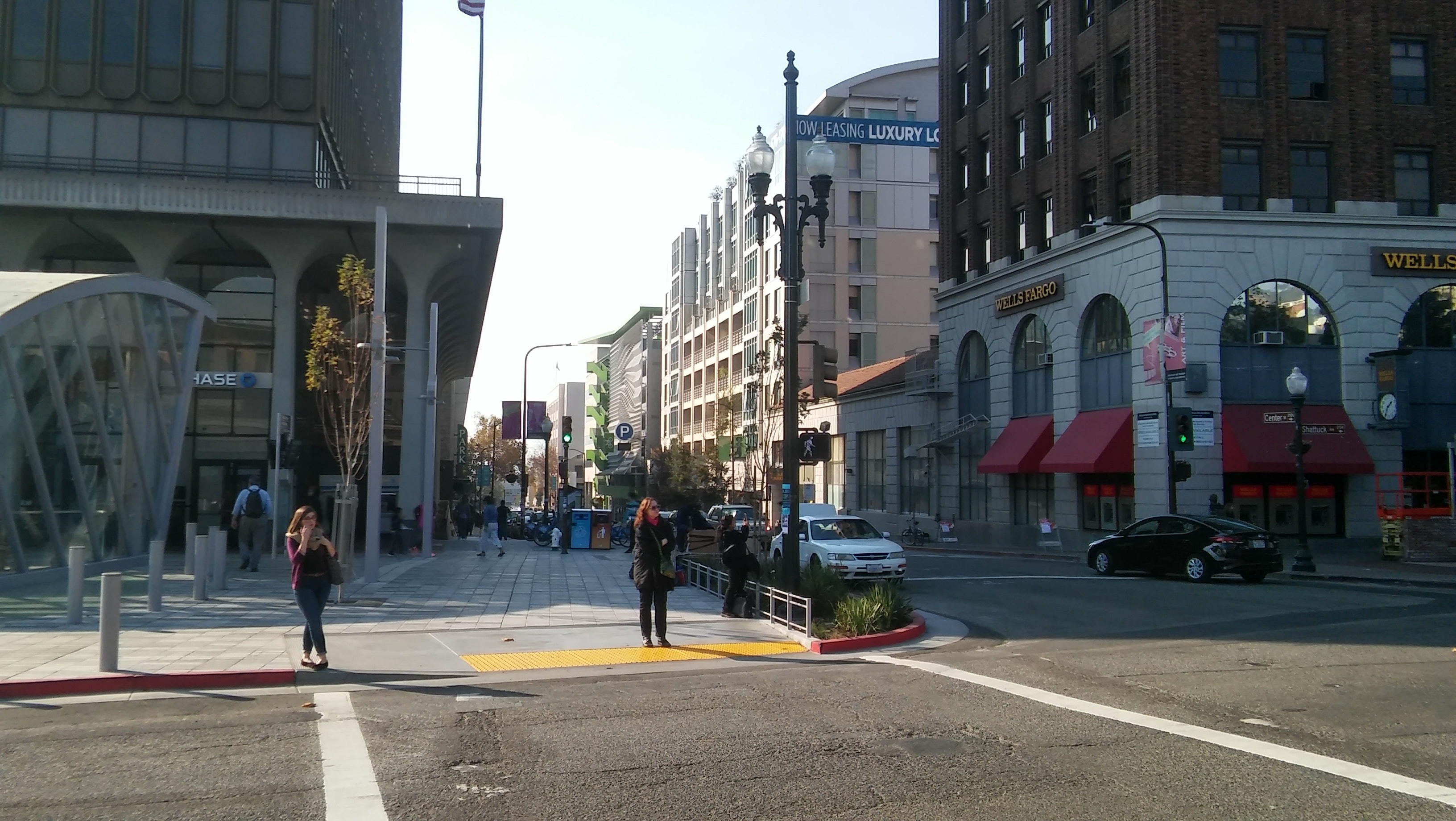
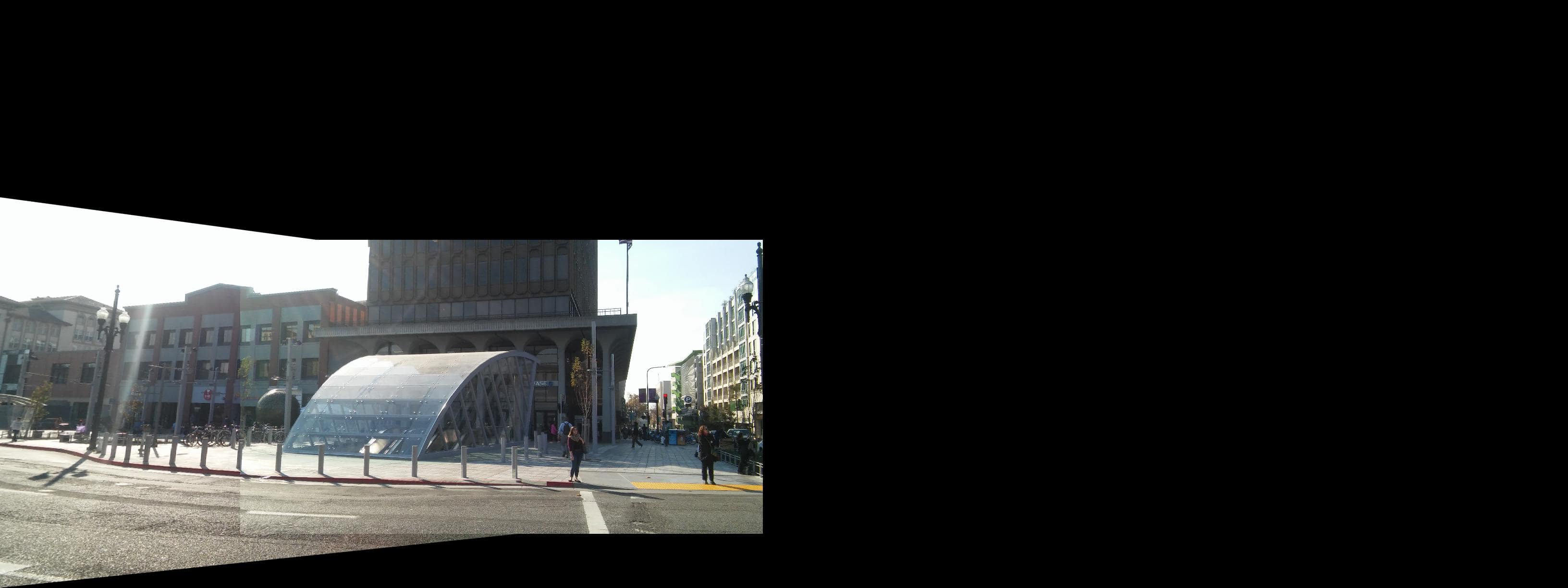
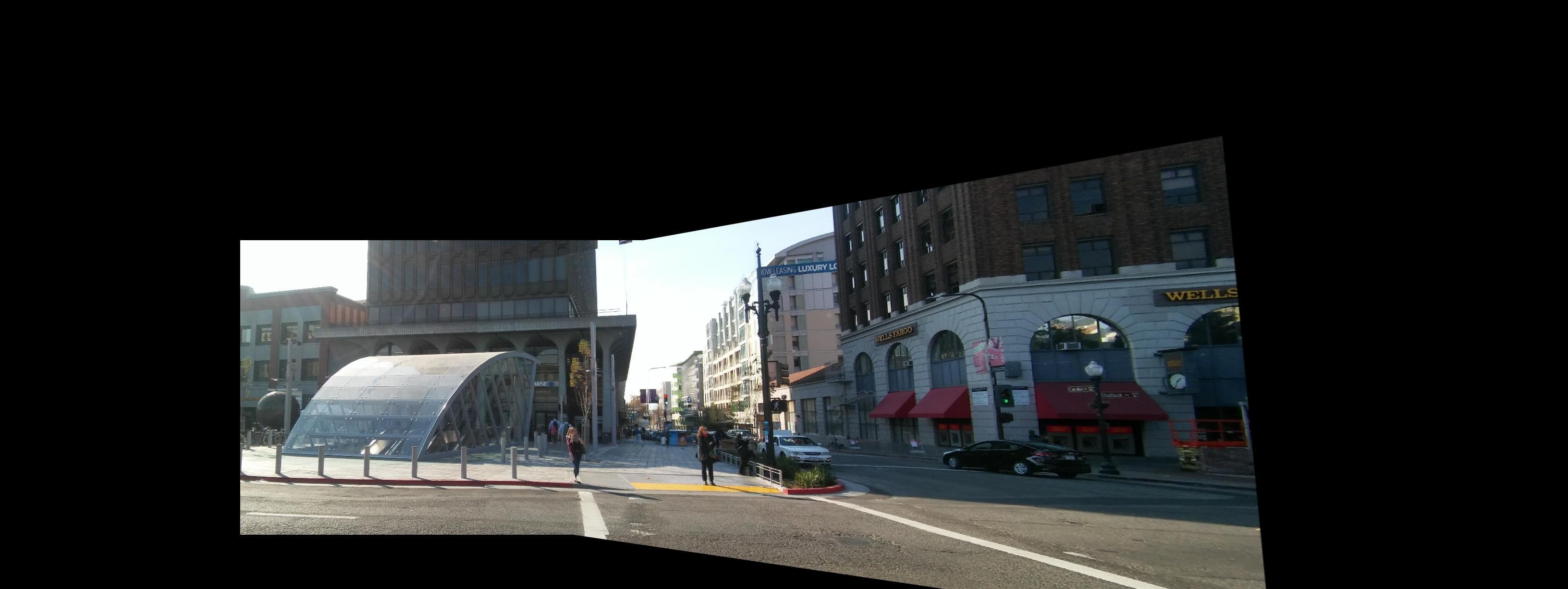
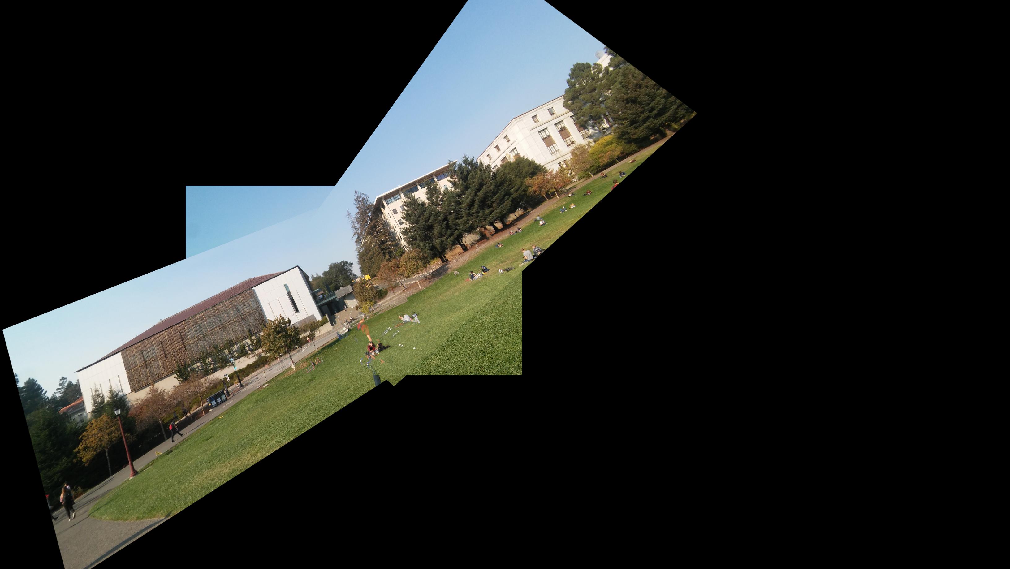
For this part of the project we are going to stitch a few images into a mosaic. The idea is to define several corresponding points between the images. I used 3 images for this part and I had two sets of corresponding points for the first and second images, and the second and third images. The first set of points are for approximating the first homography matrix using the least squares. After calculating the homography we stitch the first two images together. Then we repeat the same logic and actions to stitch the third one on the already warped image. For combining the warped images, I used the element-wise maximum of the warp images, which gave better results than linear blending.
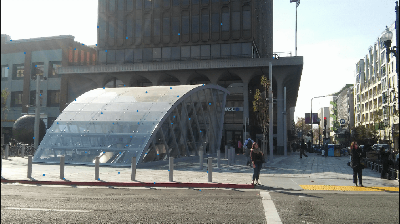
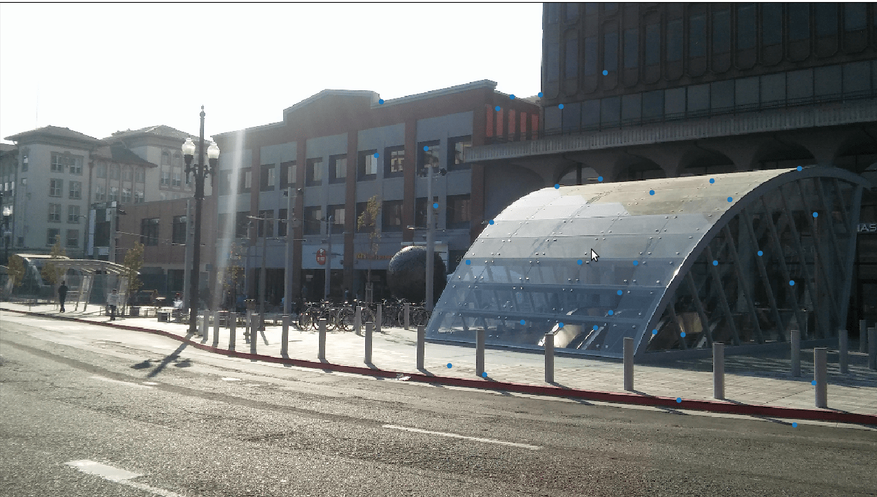
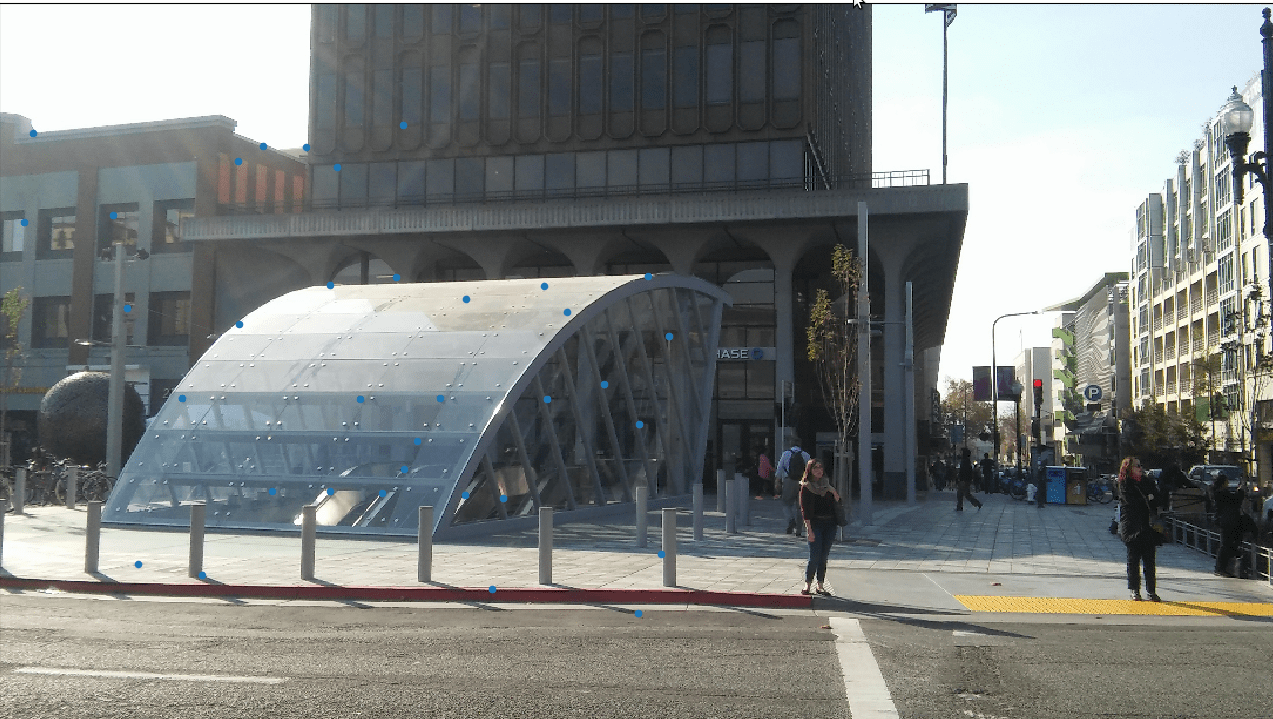
These are the 3 images from downtown berkeley Bart station.Downtown Berkeley
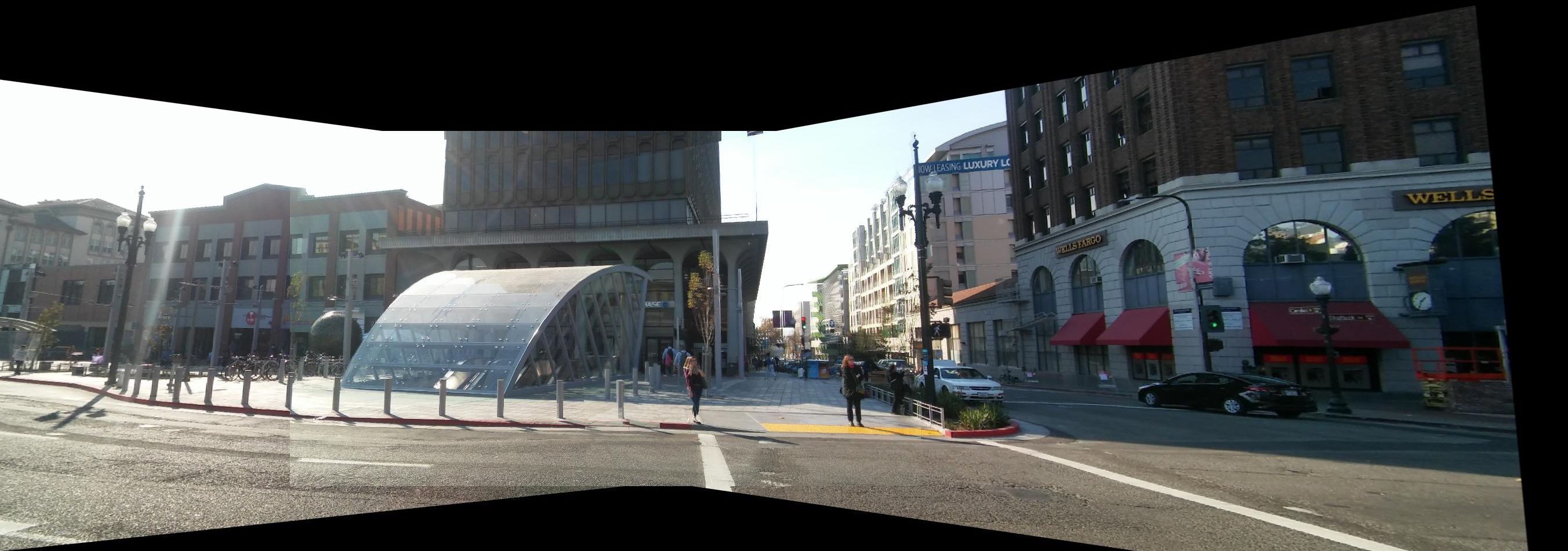
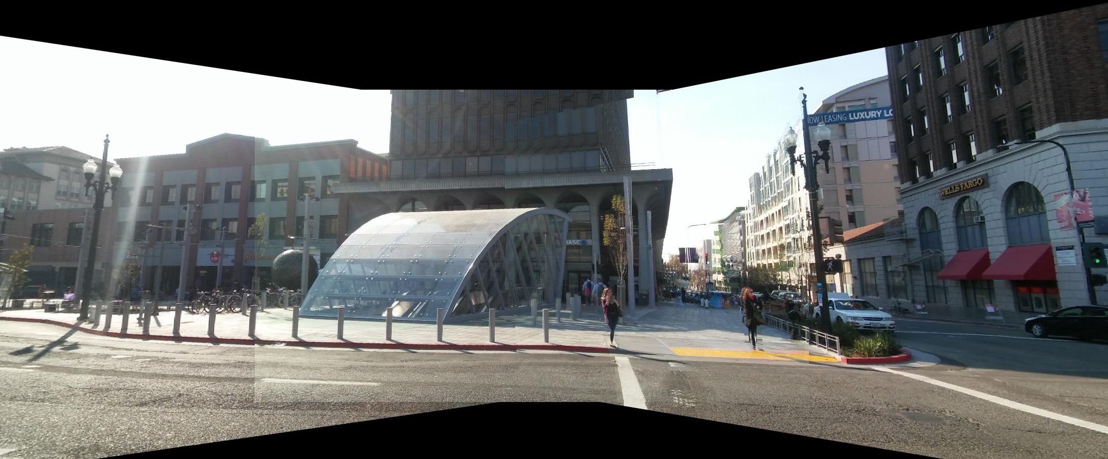
Downtown Berkeley Mosaic of 12 and 23
Downtown Berkeley Mosaic
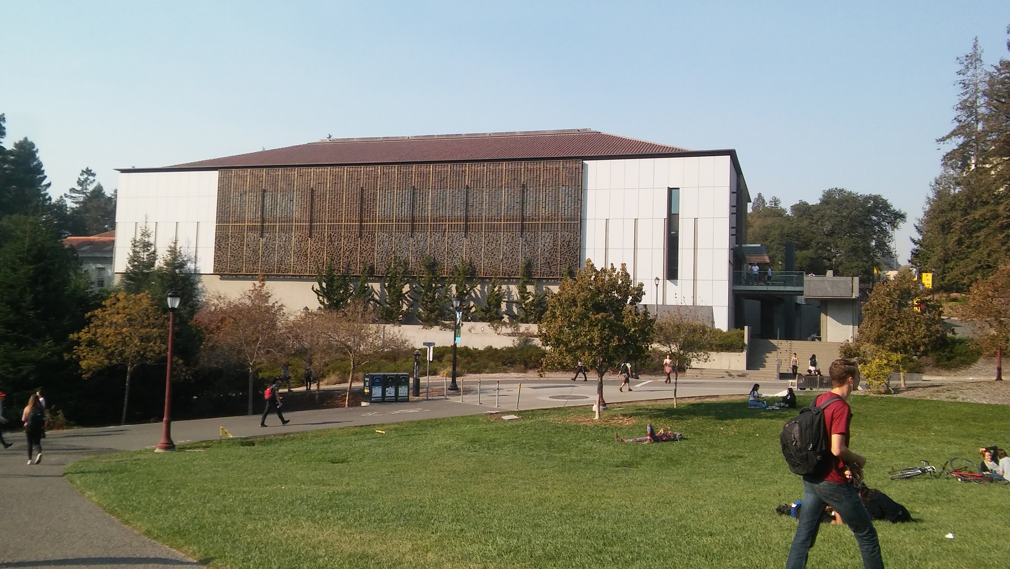
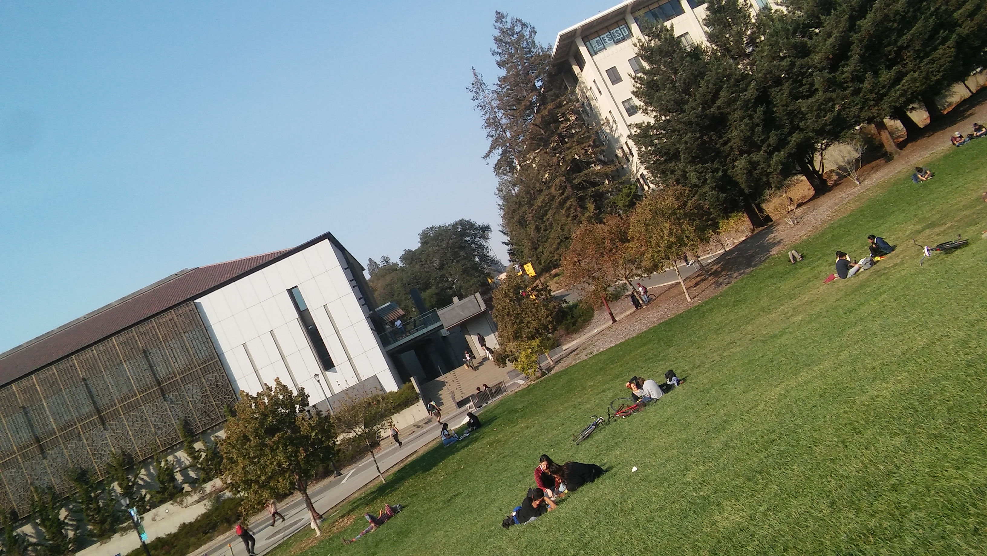
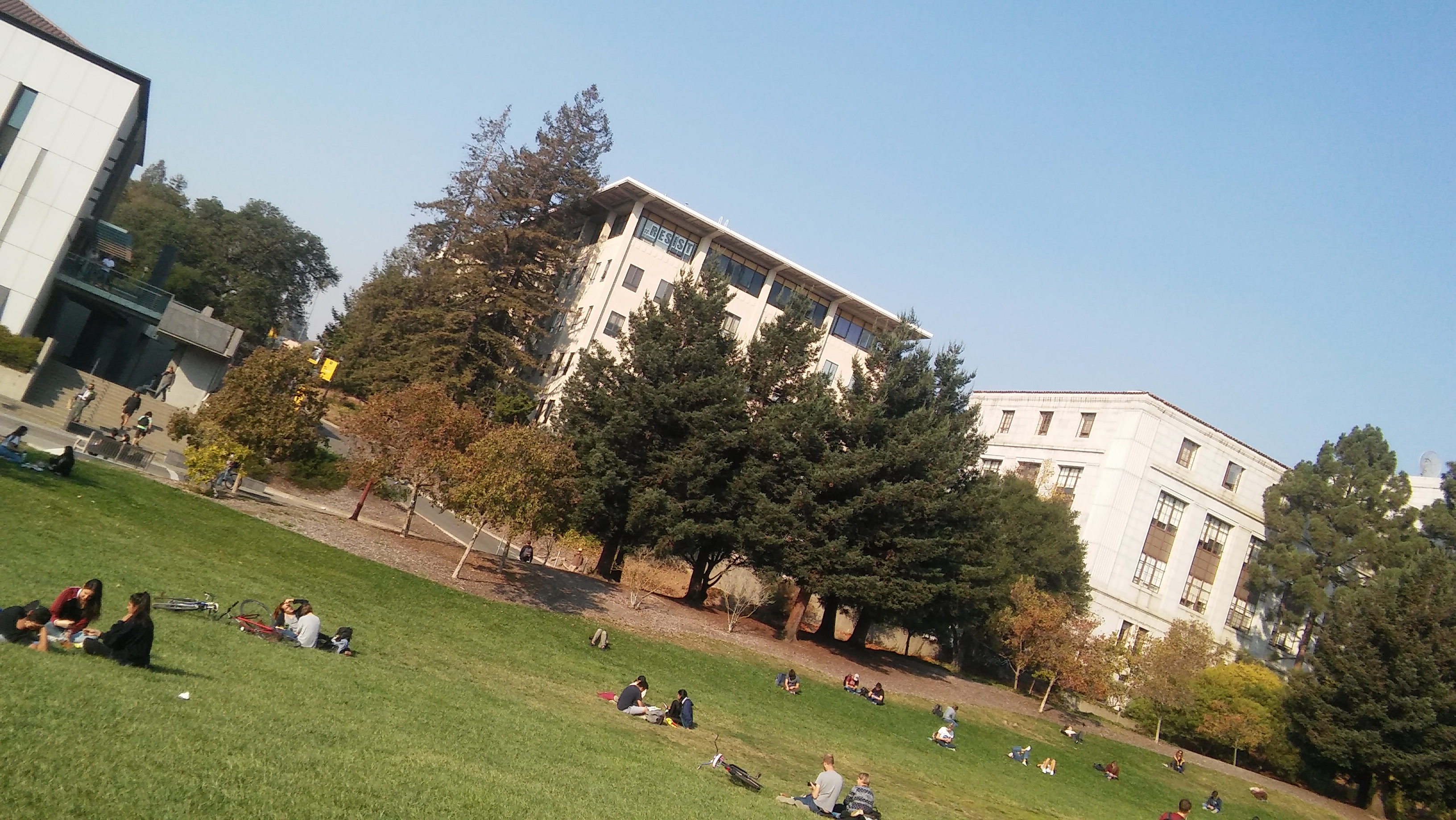
The Memorial Glade
Downtown Berkeley Mosaic
Part B
The goal of this part is to create a system for automatically stitching images into a mosaic.Harris Interest Points
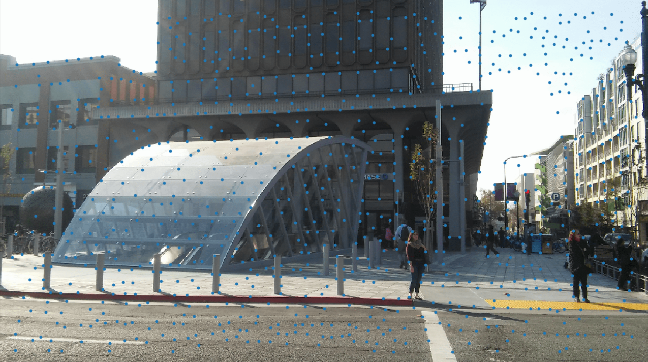
In order to find all the corner points in the image, we begin our process by finding Harris interest points. Here are example images:
Downtown Berkeley

Adaptive Non-Maximal Suppression
In order to find all the corner points in the image, we begin our process by finding Harris interest points. Here are example images: After finding the necessary Harris interest points, we want to have a good spread of the interest points, as Harris points can be concentrated near the edges and corners. For this reason, we implement Adaptive Non-Maximal Suppression and pick top 500 points from Harris corners. Here are some example images, where you can see a better distribution of the points.
Downtown Berkeley


Feature Descriptor and Feature Matching
Now we have a good distribution of interest points in both of our images and want to find the corresponding matches of those images. In part A, we did this manually, by selecting the points in both of the images. In this part, however, we implement Feature Descriptor extractor, which extracts 8x8 patches from 40x40 window of blurred descriptors and matches the corresponding patches together. For matching the features, we basically compute the distance between 64x1 size vectors and pick the closest one for each of the patches. This step gives us mapping of interest points. You can see image examples below.
Downtown Berkeley

RANSAC
As you can see in the first image above, there are some points on the left that should not have corresponding points in the right images, but unfortunately, the feature matcher finds correspondences for them as well. In order to get rid of those interest points, we implement RANSAC where we randomly pick 4 points, compute the homography and check whether the error of the other points falls below a certain threshold.
Downtown Berkeley
Autostitching
After finding the points, the rest is just the same as we did in part A. We find the closest homography and blend the images together. Here are some examplesDowntown Berkeley, Manual and Auto
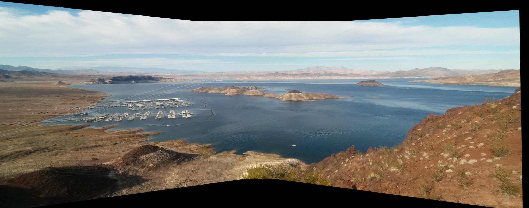
Hoover dam
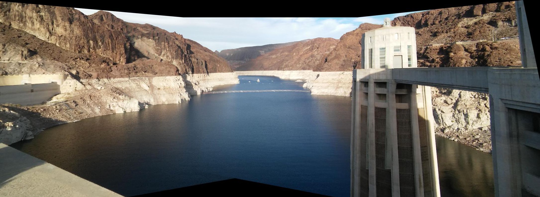
Hoover dam lake