Generally, we first define correspondence between two images. Then we can solve for a homography matrix to warp points in image 1 to corresponding points in image 2.
1. Image rectification
To rectify an image, we find 4 (or more) points which are vertices of a regular shape (optimally, a square or a rectangle). Then guess a reasonable list of coordinates which will make sense if we look at it along the normal line of the planar surface. Given these data, a projective warping could "rectify" the image.
2. Mosaic
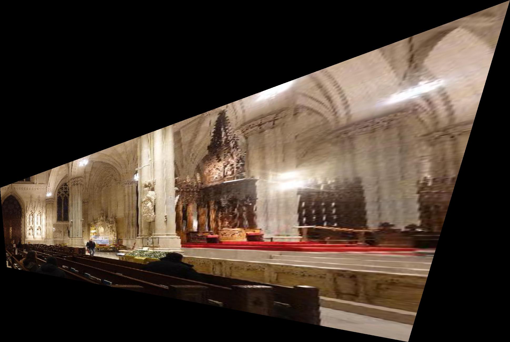
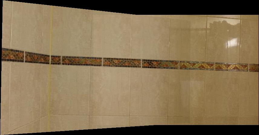
This time, we need to define a larger canvas to accommodate both images. My approach is to calculate the coordinates of four corners of image 1 after warping, compute the size of new canvas as well as the offset (as coordinates of pixels have to start from 0). And then, simply put both images on the correct position of the canvas and do a blending.
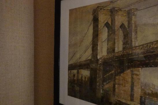
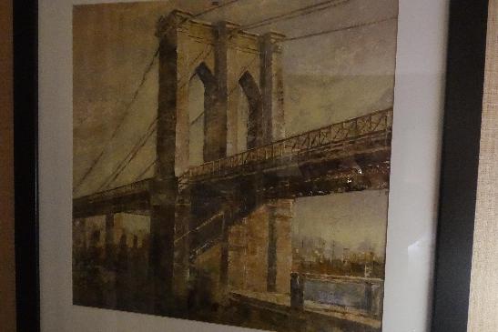
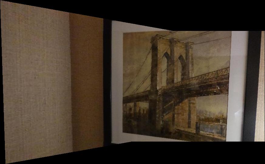
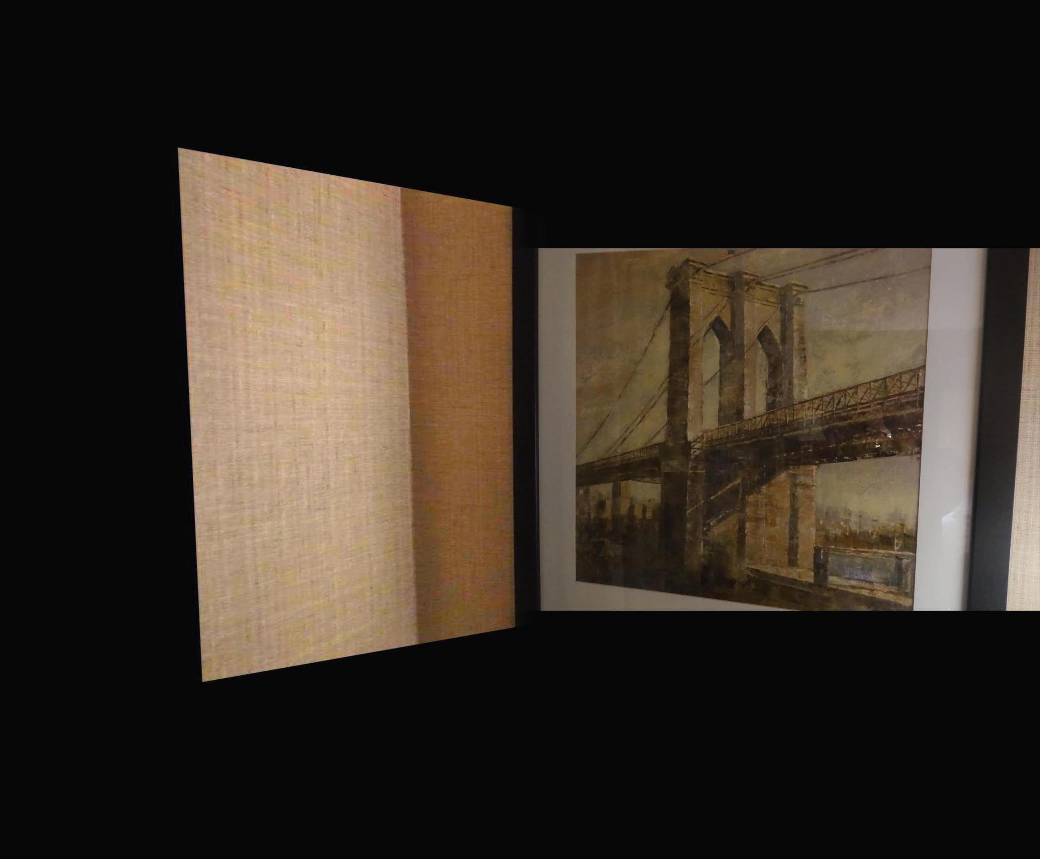
A painting of Brooklyn bridge
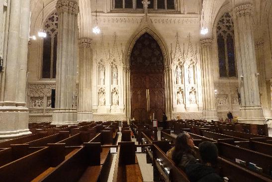
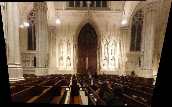
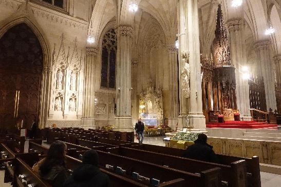
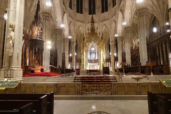
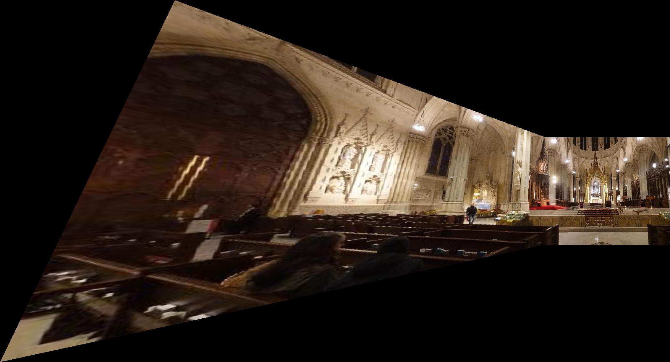
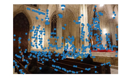
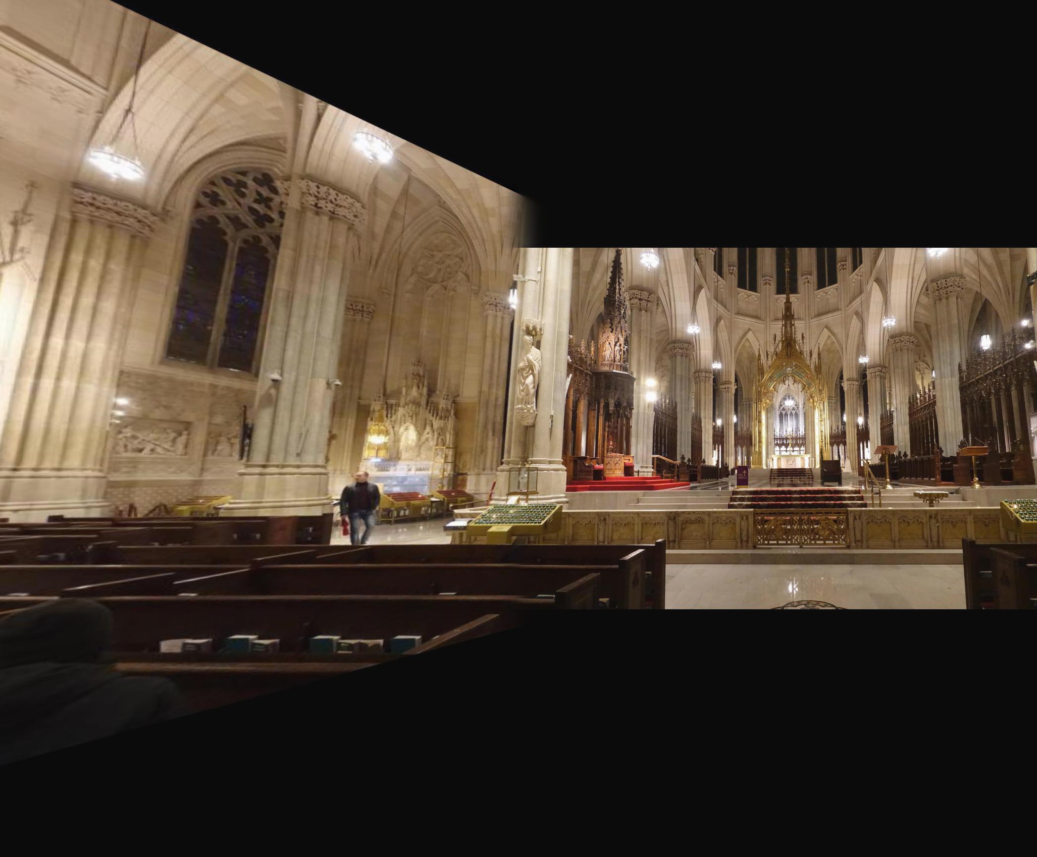
Inside St Patrick's Cathedral
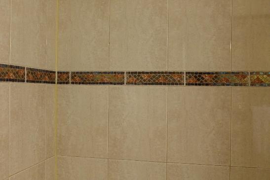
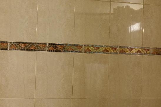
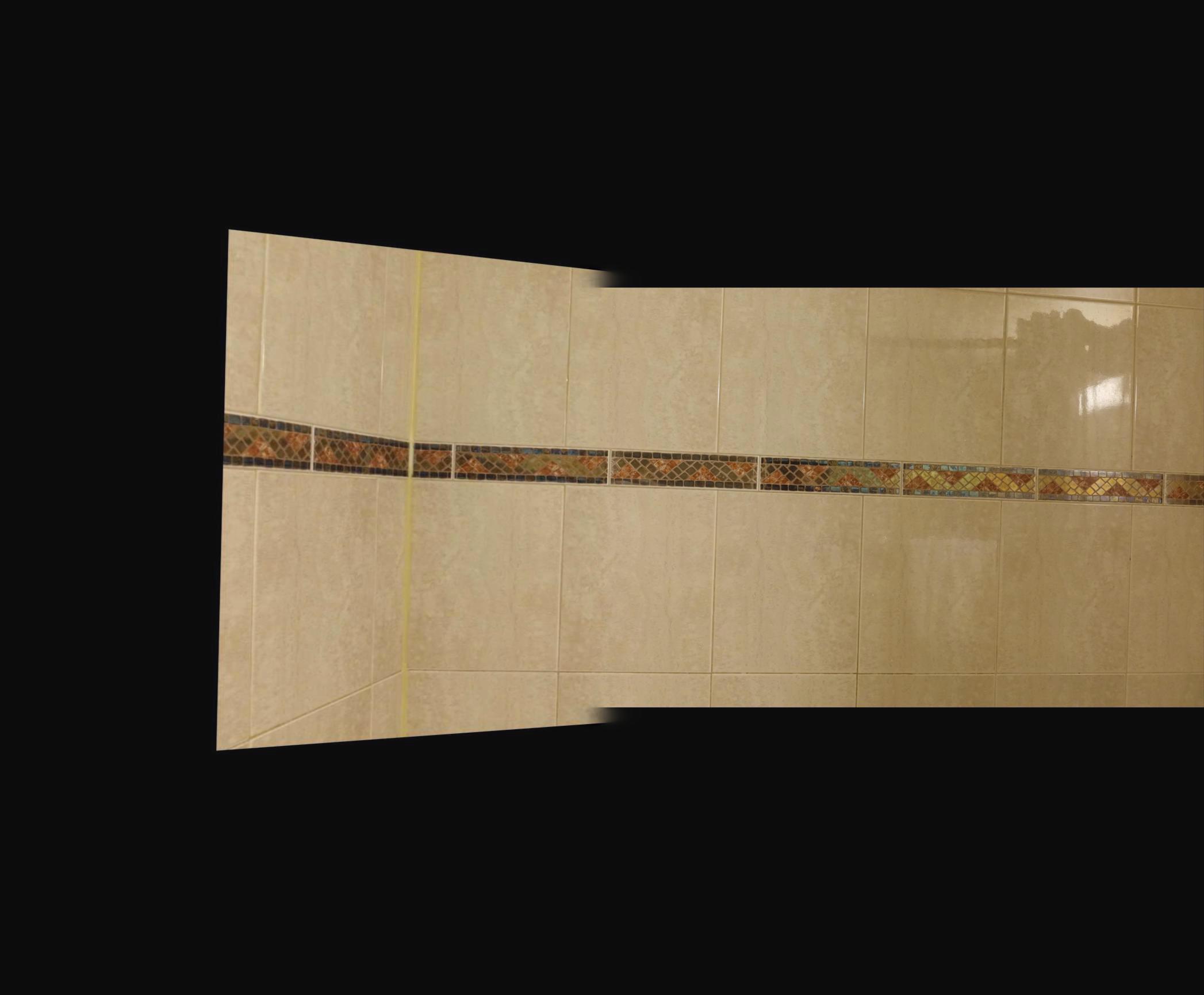
Wall of bathroom tiles
3. Summary
1. One tricky part of this project is that you have to keep center of projection unchanged when taking pictures (or, take photos of scenes far away). Otherwise, there will be pretty obvious shadows in the overlapping region.
2. At first, I was going to find a generic alpha mask to blend two images after warping. Such general mask could be hard to generate. An easy way, however, is just to have a vertical border, do a simple alpha blending, and only keep a maximal upright rectangle.
3. Projecting to a plane probably won't work for generating long panorama (like the one in iPhone Camera app), because the images on the side will be stretched a lot and lose all the details.
4. If all parameters of both images are the same, then most likely we don't need to worry about blending even if we use the simplest "taking average in the overlapping region".
Part 2: Automatic Stitching
Manually selecting correspondence could be time consuming and tedious for humans. We would like to follow the paper, “Multi-Image Matching using Multi-Scale Oriented Patches” by Brown et al., and implement a simplified version to automatically selecting correspondence in multiple images.
Harris Interest Point Detector
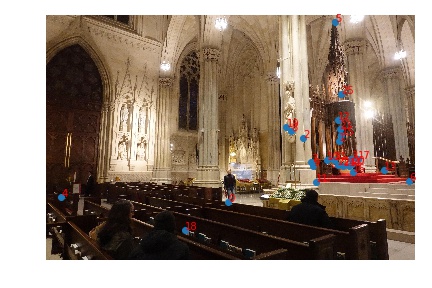
The first step is to find candidate interesting points. I used Harris Interest Point Detector for the task. skimage.feature.corner_harris is to generate a response matrix, in which a higher value indicates higher probability to be a corner. skimage.feature.peak_local_max is used to select a set of local maximum. Here we can vary the parameter, min_distance, to control the number of points selected, so that there are points spread across the whole image and also the next step (ANMS) won't execute forever.
Adaptive Non-Maximal Suppression
As you can see, Harris Detector gives us points way more than we need. So we need to take only a subset of all Harris corners. Meanwhile, we would like the remaining points to be spatially evenly distributed. The algorithm presented in the paper, ANMS, comes in handy in this situation. In a word, ANMS selects points with the largest minimum suppression radius.
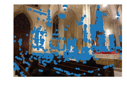
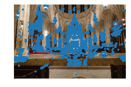
 In the formula above, I is the set of all interest points, and f is the corner response matrix we obtained in last step. I set c_robust=0.9 and keep top 500 interest points with high values of r_i. The points left are shown below.
Feature Descriptor extraction
Now each image has 500 points. How do we find the correspondence? We can generate a feature descriptor for each interest points, and find the closest match for each point. To achieve that goal, we need to define feature descriptor and a similarity measure.
For every point, I extract a 40x40 window around it, downsize it to 8x8 to get rid of high frequency signals. Then, I bias/gain normalize the descriptor by substracting the mean and dividing by standard deviation so that the descriptor is invariant to affine changes in intensity.
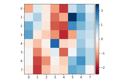
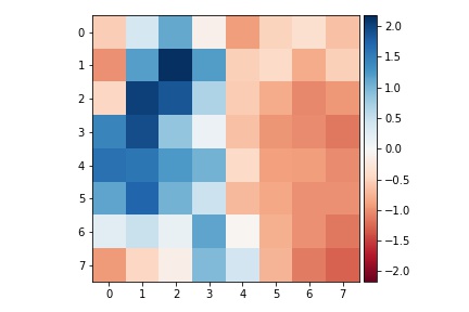
Below are two sample descriptors for the points in the image church-left.
Feature Matching
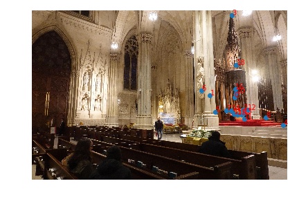
We want to find descriptors that are similar which indicate two points are likely to be a pair of correspondence. We proceed by the following algorithm: For every interest point in image1, find the nearest neighbor (1NN) and second nearest neighbor (2NN) among the set of interest points of image2. If the ratio of distance-to-1NN to distance-to-2NN is smaller than a threshold (I set 0.5), then we say the pair is a match. The rationale is that a true match should be unique and way better than other potential matches.
RANSAC
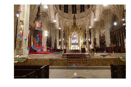
From the pictures above, we can see that there are still some outliers. Since Least Squares homography computation is sensitive to outliers, we need to filter them out before feeding the points correspondence to that step. We consider Random Sample Consensus (RANSAC) algorithm to find the true homographic transformation matrix H.
Each time, we randomly pick four pairs of points without replacement, and calculate a unique H (Eight equations for eight degrees of freedom). Then we warp all points of image1 to image2 by applying H. Define inliers to be those point pairs, in which warping the point in image 1 will take it very close to the point in image 2. Repeat the process above for many iterations, and keep the longest inliers list. In the end, using all points in the inliers list to compute the final H.
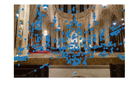
After some experiments, I set error_threshold=4, iteration=200. The points left after RANSAC are shown below.
Results
Comparing the results from automatically defined correspondence (left) and manually defined correspondence (right).
 As we can see, the automatic correspondence generates satisfying results. The only noticable imperfection is in the church mosaic (First row, left), in which the benches do not line up perfectly. However, I believe given more iterations and smaller error threshold in RANSAC, the mosaic could be improved.
Summary
Automatical alignment needs to be robust and precise. To be robust, we need to first provide enough corners as candidates for correspondence. To be precise, we need to filter out incorrect correspondence while keeping running time and memory in mind.
The intuition of building descriptors as described in this report is that high frequency signals usually mess around with SSD. So to find a matching, we can build descriptors based on low frequency signals.
A painting of Brooklyn bridge
Inside St Patrick's Cathedral
Wall of bathroom tiles
3. Summary
1. One tricky part of this project is that you have to keep center of projection unchanged when taking pictures (or, take photos of scenes far away). Otherwise, there will be pretty obvious shadows in the overlapping region.
2. At first, I was going to find a generic alpha mask to blend two images after warping. Such general mask could be hard to generate. An easy way, however, is just to have a vertical border, do a simple alpha blending, and only keep a maximal upright rectangle.
3. Projecting to a plane probably won't work for generating long panorama (like the one in iPhone Camera app), because the images on the side will be stretched a lot and lose all the details.
4. If all parameters of both images are the same, then most likely we don't need to worry about blending even if we use the simplest "taking average in the overlapping region".
Part 2: Automatic Stitching
Manually selecting correspondence could be time consuming and tedious for humans. We would like to follow the paper, “Multi-Image Matching using Multi-Scale Oriented Patches” by Brown et al., and implement a simplified version to automatically selecting correspondence in multiple images.
Harris Interest Point Detector
The first step is to find candidate interesting points. I used Harris Interest Point Detector for the task. skimage.feature.corner_harris is to generate a response matrix, in which a higher value indicates higher probability to be a corner. skimage.feature.peak_local_max is used to select a set of local maximum. Here we can vary the parameter, min_distance, to control the number of points selected, so that there are points spread across the whole image and also the next step (ANMS) won't execute forever.
Adaptive Non-Maximal Suppression
As you can see, Harris Detector gives us points way more than we need. So we need to take only a subset of all Harris corners. Meanwhile, we would like the remaining points to be spatially evenly distributed. The algorithm presented in the paper, ANMS, comes in handy in this situation. In a word, ANMS selects points with the largest minimum suppression radius.
In the formula above, I is the set of all interest points, and f is the corner response matrix we obtained in last step. I set c_robust=0.9 and keep top 500 interest points with high values of r_i. The points left are shown below.
Feature Descriptor extraction
Now each image has 500 points. How do we find the correspondence? We can generate a feature descriptor for each interest points, and find the closest match for each point. To achieve that goal, we need to define feature descriptor and a similarity measure.
For every point, I extract a 40x40 window around it, downsize it to 8x8 to get rid of high frequency signals. Then, I bias/gain normalize the descriptor by substracting the mean and dividing by standard deviation so that the descriptor is invariant to affine changes in intensity.
Below are two sample descriptors for the points in the image church-left.
Feature Matching
We want to find descriptors that are similar which indicate two points are likely to be a pair of correspondence. We proceed by the following algorithm: For every interest point in image1, find the nearest neighbor (1NN) and second nearest neighbor (2NN) among the set of interest points of image2. If the ratio of distance-to-1NN to distance-to-2NN is smaller than a threshold (I set 0.5), then we say the pair is a match. The rationale is that a true match should be unique and way better than other potential matches.
RANSAC
From the pictures above, we can see that there are still some outliers. Since Least Squares homography computation is sensitive to outliers, we need to filter them out before feeding the points correspondence to that step. We consider Random Sample Consensus (RANSAC) algorithm to find the true homographic transformation matrix H.
Each time, we randomly pick four pairs of points without replacement, and calculate a unique H (Eight equations for eight degrees of freedom). Then we warp all points of image1 to image2 by applying H. Define inliers to be those point pairs, in which warping the point in image 1 will take it very close to the point in image 2. Repeat the process above for many iterations, and keep the longest inliers list. In the end, using all points in the inliers list to compute the final H.
After some experiments, I set error_threshold=4, iteration=200. The points left after RANSAC are shown below.
Results
Comparing the results from automatically defined correspondence (left) and manually defined correspondence (right).
As we can see, the automatic correspondence generates satisfying results. The only noticable imperfection is in the church mosaic (First row, left), in which the benches do not line up perfectly. However, I believe given more iterations and smaller error threshold in RANSAC, the mosaic could be improved.
Summary
Automatical alignment needs to be robust and precise. To be robust, we need to first provide enough corners as candidates for correspondence. To be precise, we need to filter out incorrect correspondence while keeping running time and memory in mind.
The intuition of building descriptors as described in this report is that high frequency signals usually mess around with SSD. So to find a matching, we can build descriptors based on low frequency signals.