CS 194-26: Image Manipulation and Computational Photography

Project 6: Stitching Photo Mosaics

Ryan El Khoury, CS196-26-aah

Part A: Image Warping and Mosaicing

The human field of view extends beyond what we see in traditional photos. Mosaics are a way we can approach this wide field of view. Photos are taken starting from the left or right side, rotating the camera by a little for each entry in the mosiac. For the process to work, the camera must remain in the same physical position in world space. This because the aligning and stitching of the images together requires projective warping the images so they are all on the same plane. The alignment does require the distortion of some of the scene (just like a wide angle lens) but the result is a clean overlap between the shared features in the images.

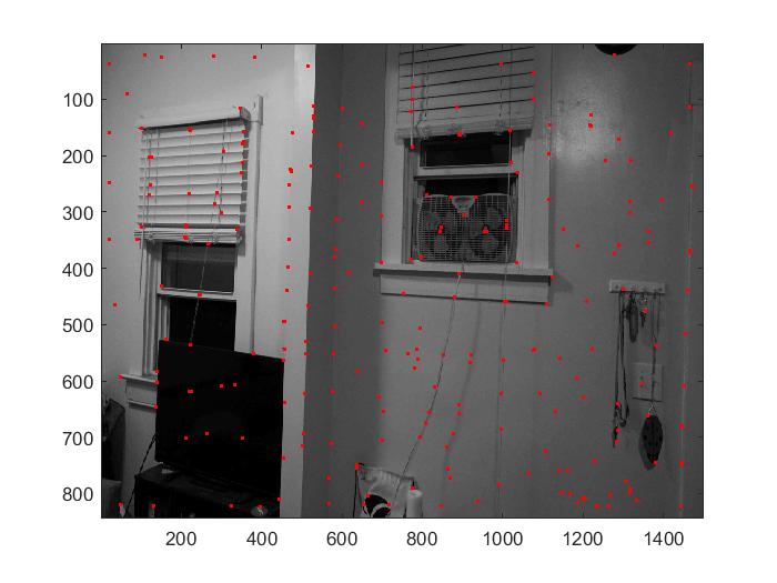
Shooting the Pictures & Correspondence Points

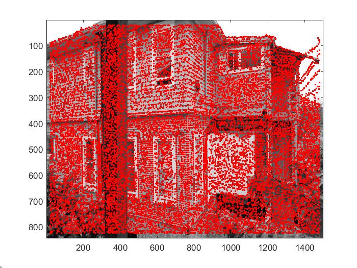
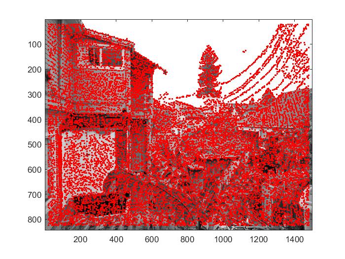
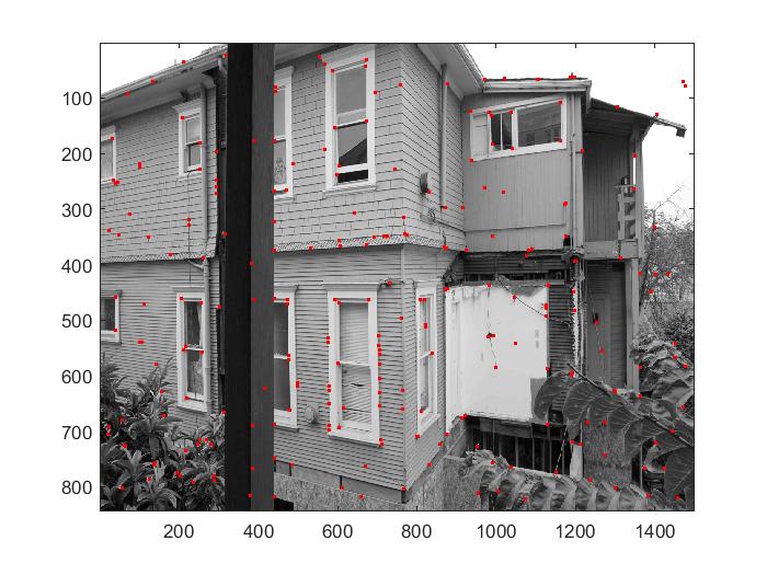
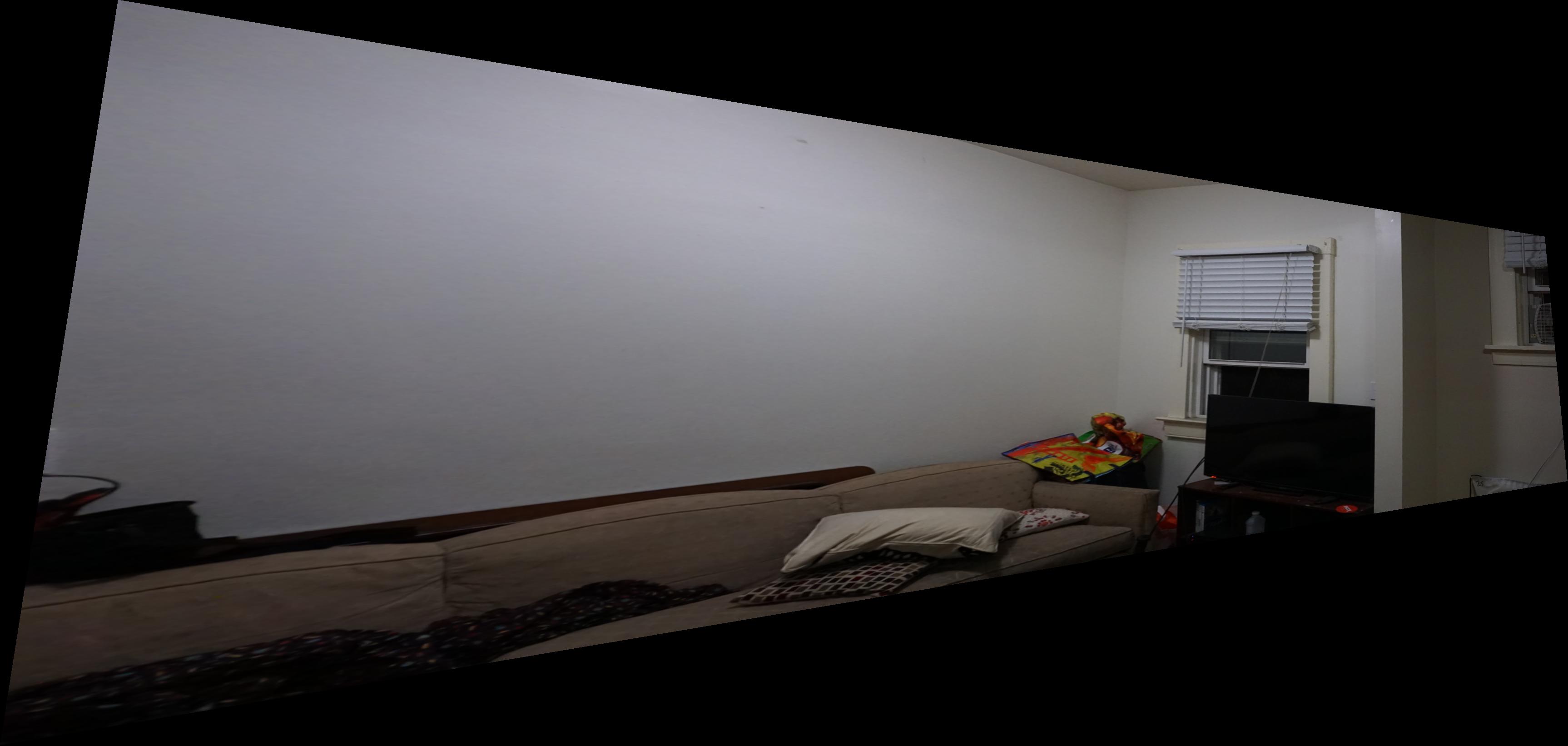
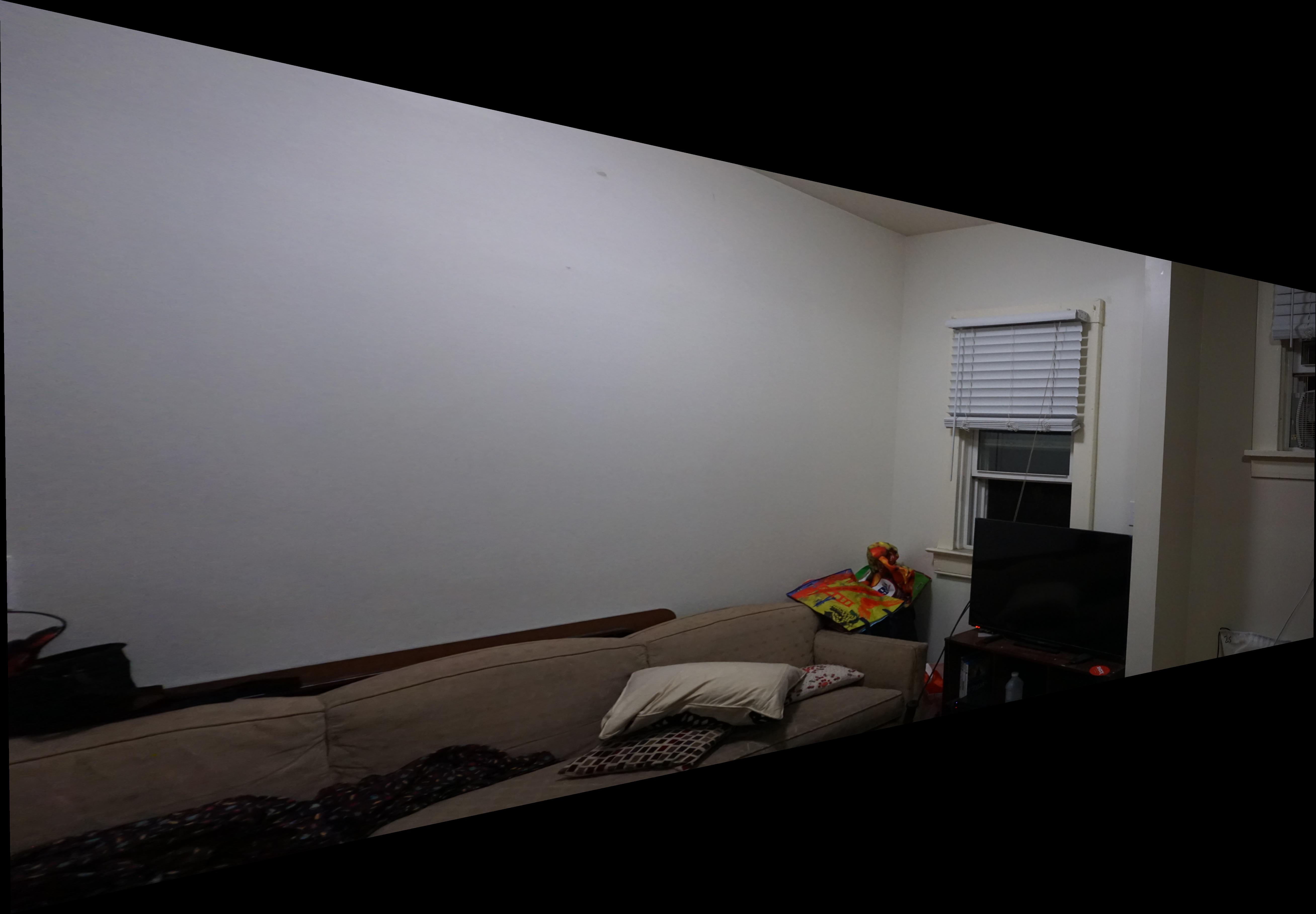
The pictures were taken on a tripod. I took a series of 7 photos for each scene starting from the left, rotating to the right by about 30 degrees for each shot. I choose two photos from each scene and identified shared features between these two. These features are demarcated with correspondence points: pairs of points meant to identify the same objects in both scenes.

Left image of interior.
Right image of interior.
Correspondence points for interior.

Recover Homographies

Once we have the correspondence points between the two images, we can calculate a transformation matrix that can change the correspondence points on one image to be on the same plane as the other. A homography is a 3 x 3 matrix with 8 degress of freedom, so we must provide at least 4 correspondence points to determine it with least squares.
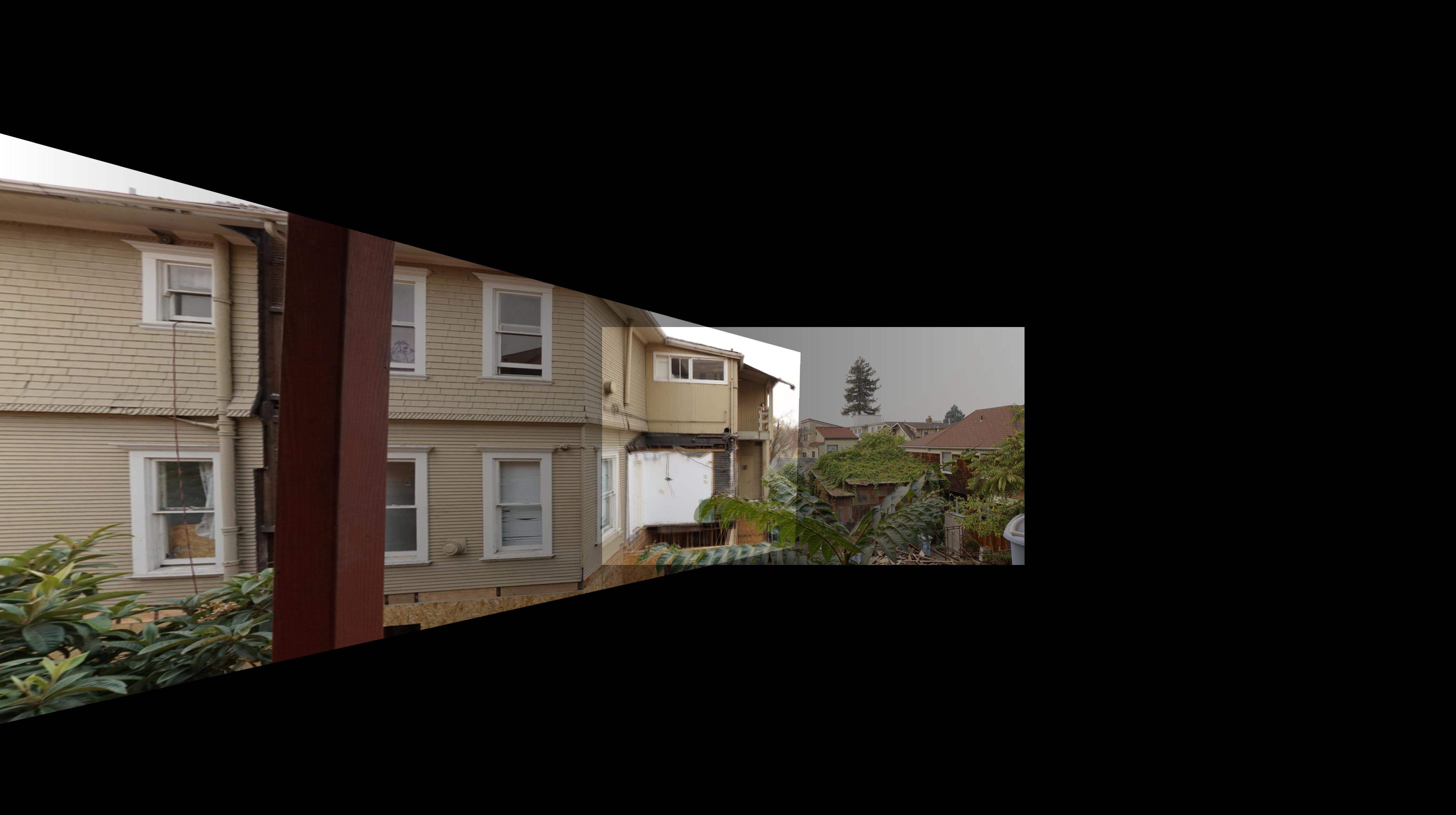
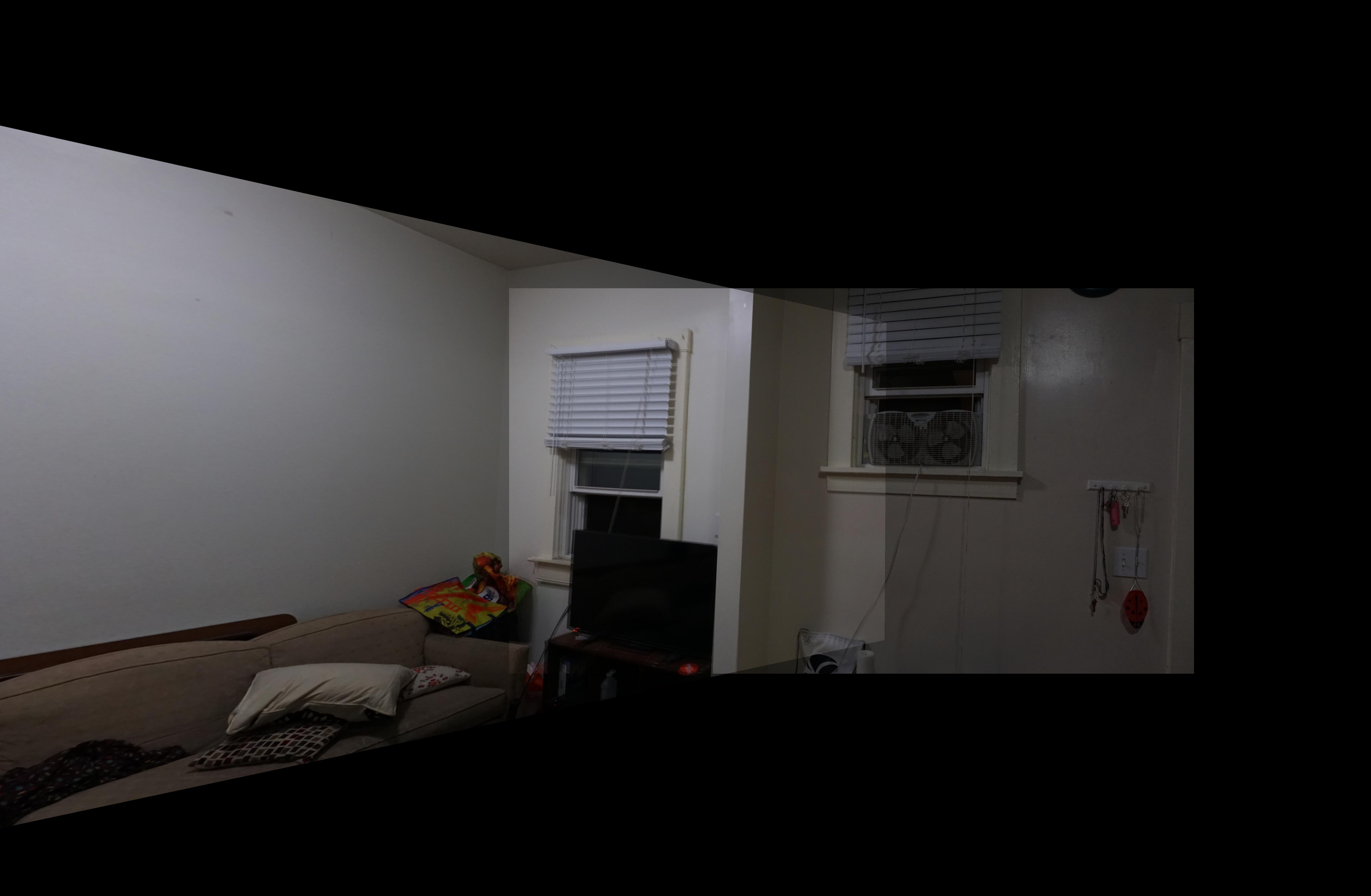
Warp the Images

Once we have the homography, we can apply it to the points from the image we want to warp to see what it would look like if it were on the plane of its partner image. The image will look distorted away from the correspondence points because it shifted to match up with the correspondence areas of the other image as much as possible. Identifying the placement of the pixels in the homography transformed image is done with inverse warping. Inverse warping consists of finding what values we should assign to the warped image by applying the inverse of the homography to the partner image. This gives us the approximate location of the unwarped source image that we should interpolate from to end up with our warped image.
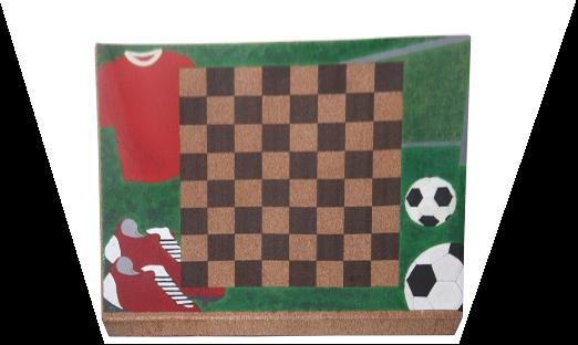
Left image of interior (to be warped).
Warped image.

Image Rectification

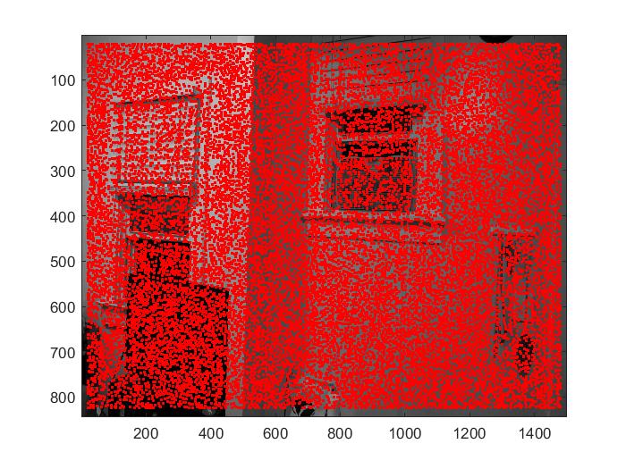
Rectification takes advantage of the warping properties of homographies to morph an image into a specific shape/direction. The correspondence points on the other image can form a square. The end result is the image warped so the correspondence points assume a square shape.
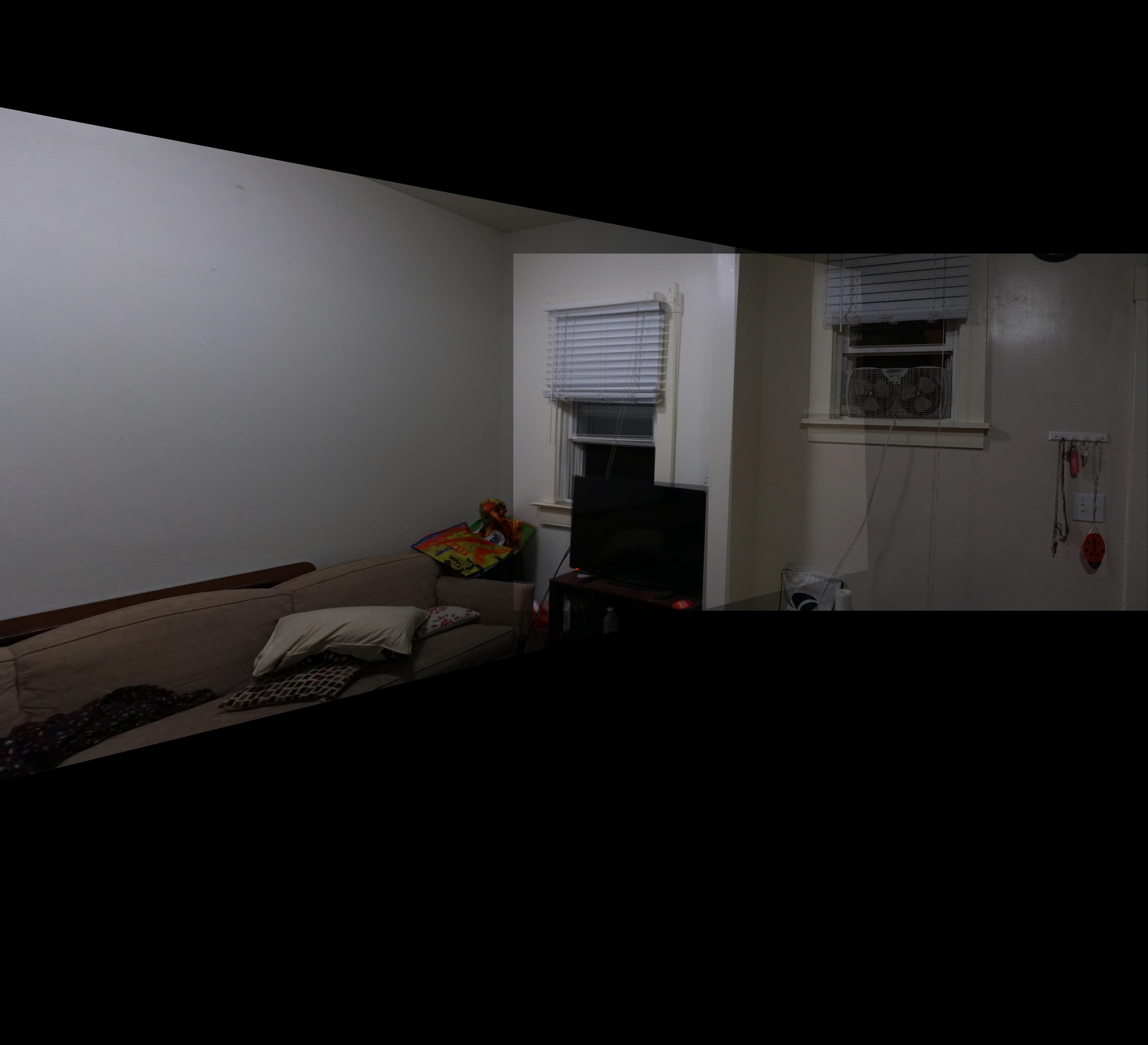
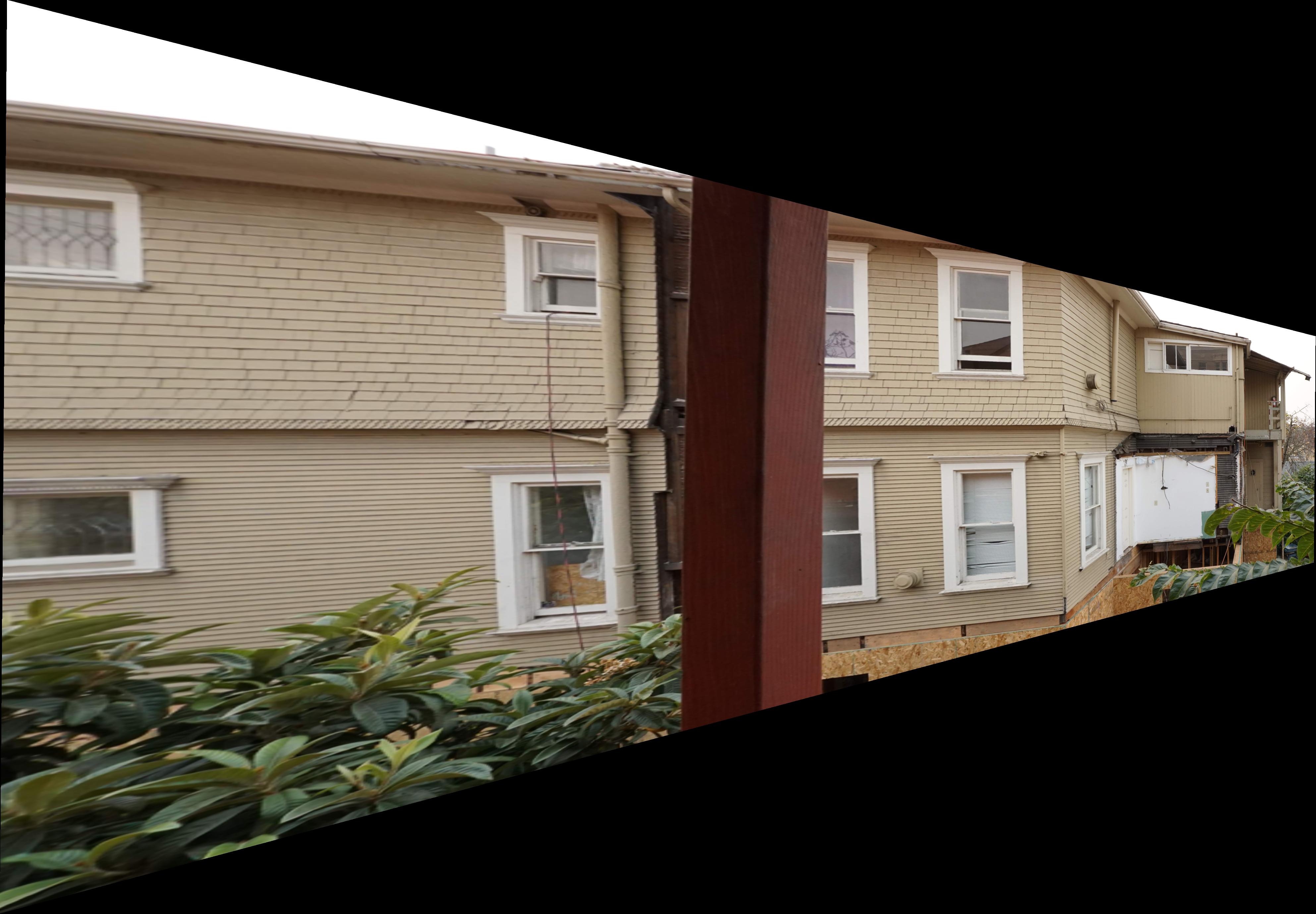
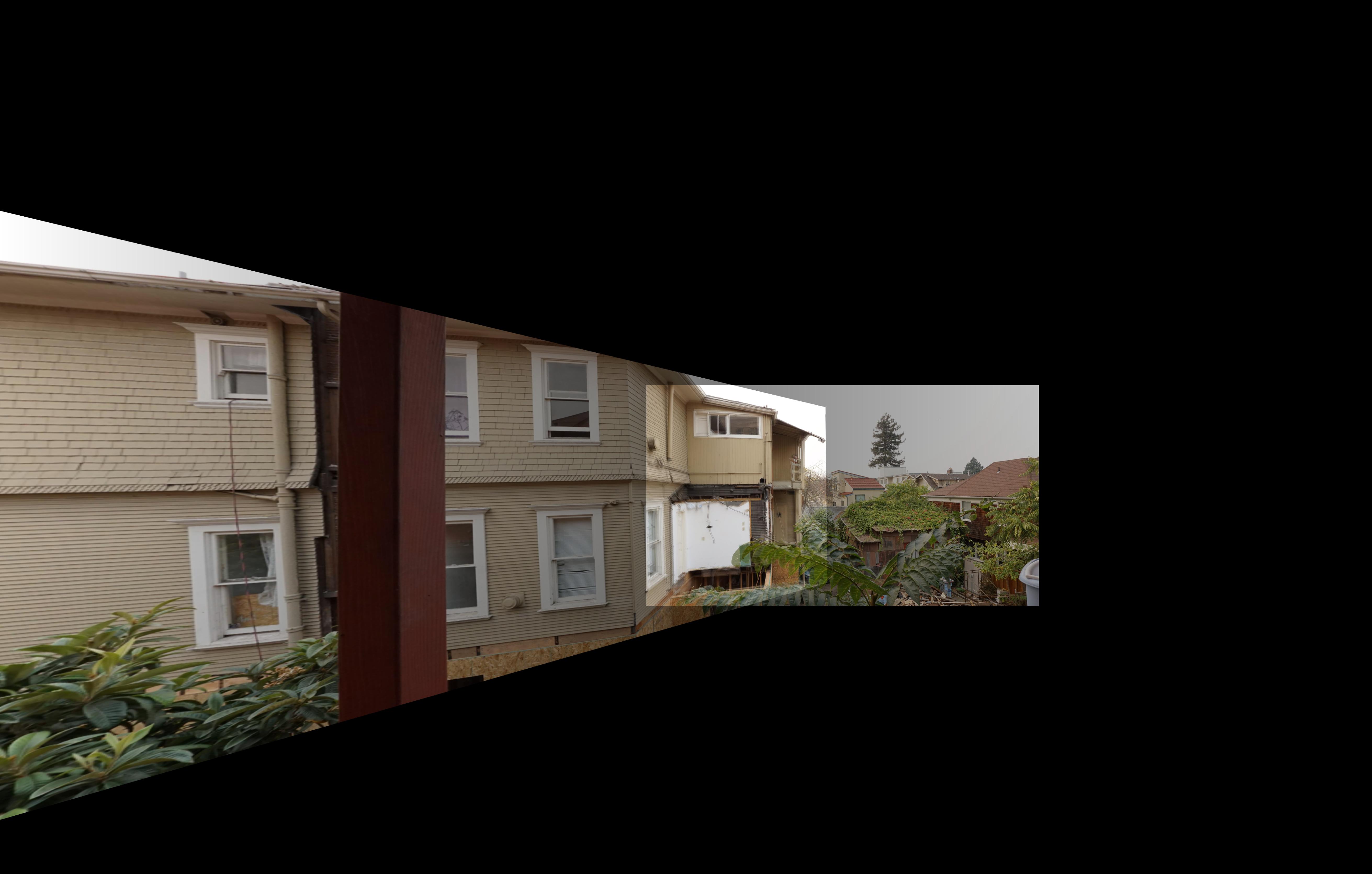
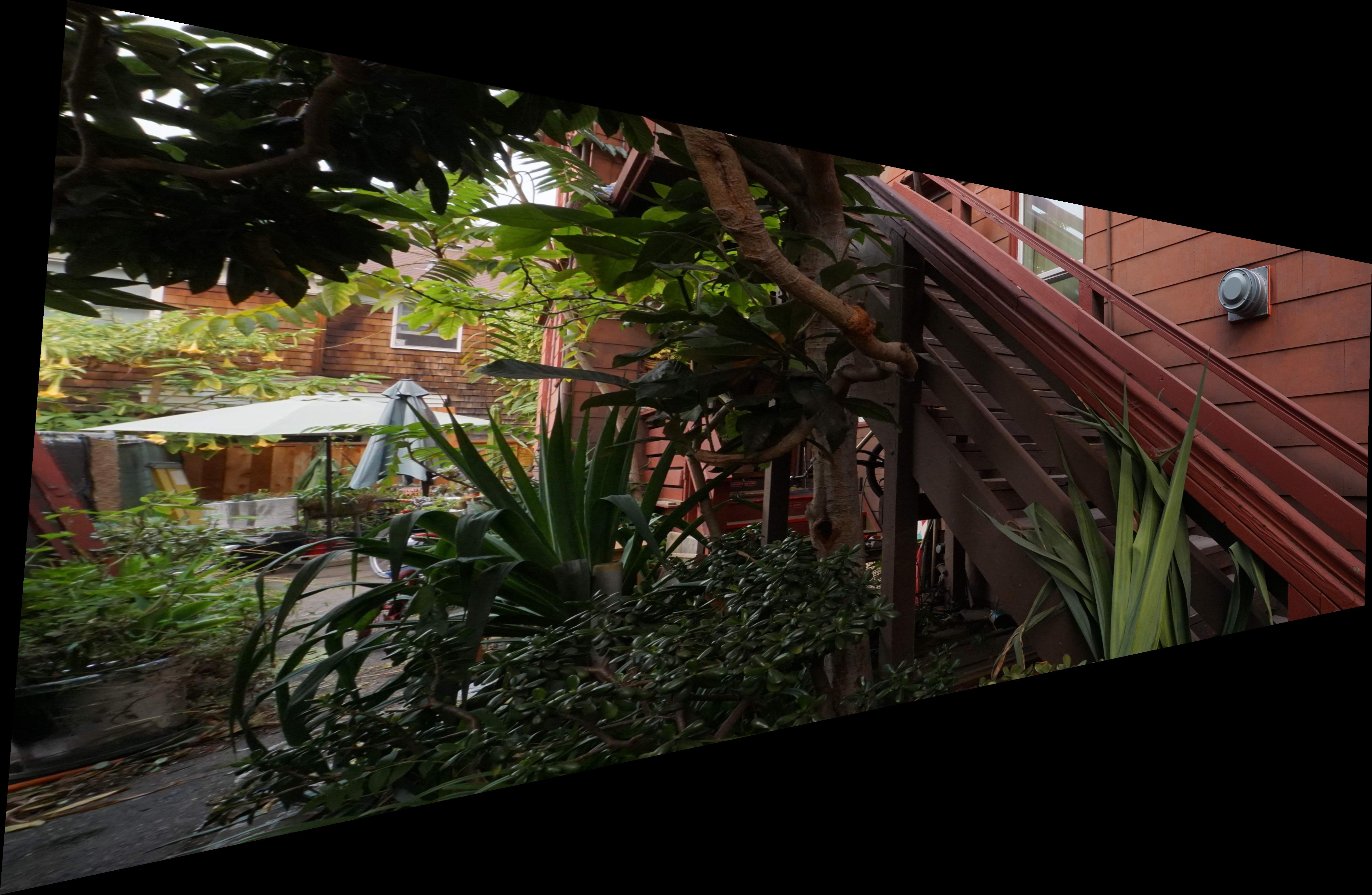
Chess board, seen from a slanted angle.
Correspondence points on chess board and intended rectification shape.
Rectified chess board.
Window/TV, seen from a slanted angle.
Correspondence points on room scene and intended rectification shape.
Rectified window/tv.

Mosaicing

Using the techniques outlines before, we can create mosiacs. We warp the left image onto the image plane of the right and stitch using Laplacian blending. The brightness of the overlapping portions of the image were probably due to imprecise averages between the two images.

Left image of interior.
Right image of interior.
Left image warped to right image plane.
Stitched interior.
Left image of balcony.
Right image of balcony.
Left image warped to right image plane.
Correspondence points picked for balcony images.
Stitched balcony.
Left image of stairs.
Right image of stairs.
Left image warped to right image plane.
Intermediate level of Laplacian blend.
Stitched stairs.

Part A Summary

The most interesting thing I learned from this part of the project was how much the information contained within an image can be shifted to give an entirely new perspective. In particular, rectifying part of an image to be "straight" not only straightens out the specified area, but also the entire image. On top of that, the result does not even look that warped/stretched!

Part B: Feature Matching for Autostitching

Picking out the correspondence points is timestaking and prone to human error. We can automate this process so the entire process can be entirely hands-off. The end result is partially determined by randomness (RANSAC) but can definitely match up to the human-guided equivalent.

Detecting Corner Features

Features are elements of an image that are discernable to the human eye. The presence of an object that makes it stand out from a scene can be detected using corner detectors. The Harris corner detector inspects each pixel and its neighbors for shifts in intensity. If the pixel has a high enough "corner response" to pass a threshold, we consider it a point of interest. The threshold for the starter code given considered a bit too many posts but that will be rectified by Adaptive Non-Maximal Suppression.

Balcony left image.
Harris corners overlaid on balcony left.
Balcony right image.
Harris corners overlaid on balcony right.

Adaptive Non-Maximal Suppression

Adaptive Non-Maximal Supression reduces the amount of interest points detected in an image in a way that ensures a good distribution across the entire image. For each interest point, the radius from its nearest, largest neighbor (in terms of corner response) is recorded. The interest points selected are ordered based on the radius size, descending. Having a large radius size means that the interest point has a high corner response and is relatively dominant in its immediate area. The dominance of a point in its area means that nearby points will have a low radius. The result after picking from the top radius interest points is a nice spread of interest points.

Harris corner features overlaid on balcony.
Balcony left image with ANMS.
Harris corners overlaid on room.
Room left image with ANMS.

Feature Descriptor and Matching

We want to create correspondences From the remaining interest points. To do this, we create 8 x 8 patches (downsampled from 40 x 40 patches) for each of the interest points. These patches are compared to each patch in the other picture to generate a map of SSD scores. The lowest SSD score is presumably the closest match to the point. But to complete the feature matching, we test whether the correspondence passes the Lowe threshold. The Lowe threshold tests the validity of the closest match by creating a threshold from the two closest nearest neighbors.

Balcony correspondence points after Lowe thresholding.

RANSAC

RANSAC stands for Random Sample Consensus. It decides a homography to compute by looking for inliers, points that match up well against its correspondance when a randomly selected homography is applied to them. The homographies we use to test for inliers are generated from 4 randomly selected correspondence points. After a number of iterations, the inlier set that was the largest contain the correspondence points we want to use to calculate the "real" homography.

Correspondence points chosen by RANSAC after 250 iterations.

Mosaic Comparison

The mosaics on the left were hand-selected and stitched while the ones on the right were computed automatically

Stitched balcony.
Auto-Stitched balcony.
Stitched interior.
Auto-Stitched interior.
Stitched stairs.
Auto-Stitched stairs.

Part B Summary

The most interesting thing I learned from this part of the project was how accurate MOPS descriptor vectors can be in determining the correspondence points between two images. On top of being able to determine the similar, significant points between images, the computer-calculated placements are probably more accurate on a pixel level than hand-selection could ever be.