Project 6: (Auto)stitching and Photo Mosaics
cs194-26-aaj
Part 1: Warping and Stitching Photos
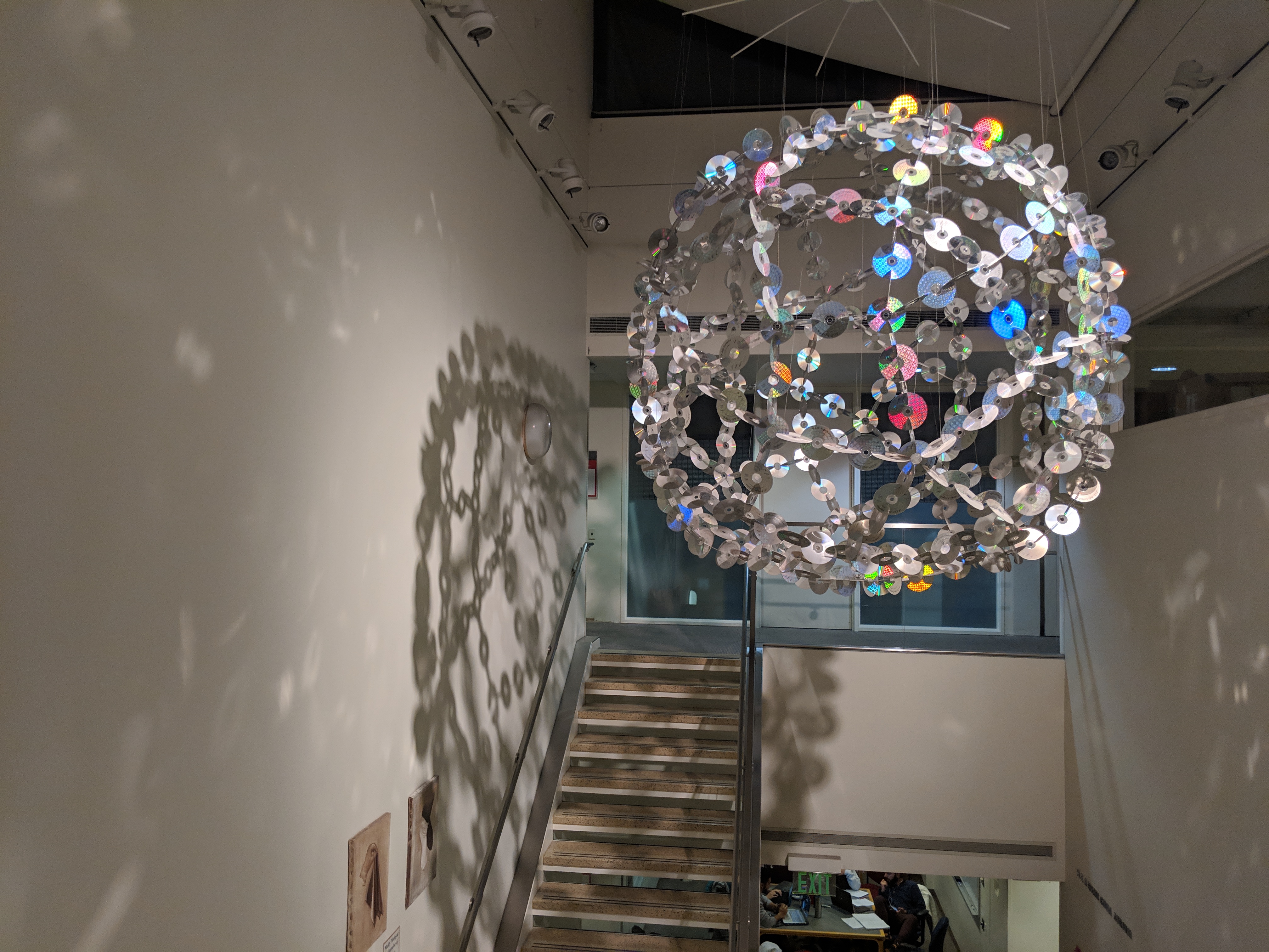
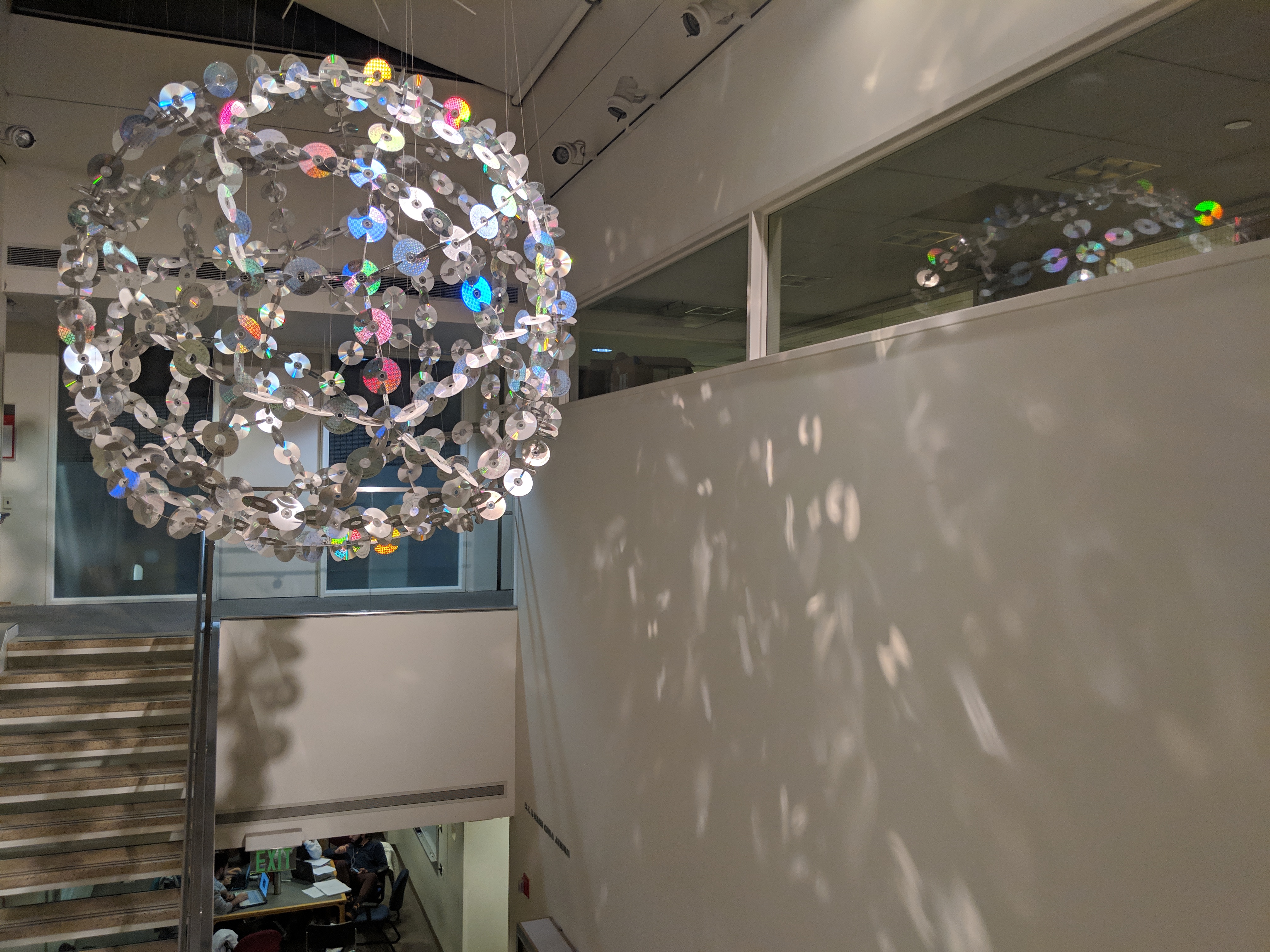
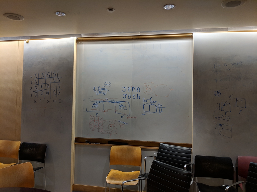
Taking photos
I took photos trying to ensure lighting was equal and sure not to translate the camera between photos, keeping a 30-60% overlap.
Calculating Homography
I first manually selected correspondence points between 2 images and then automatically calculated the homography.
I calculated the homography matrix required to transform one image to the alignment of the other by solving a system of linear equations with least squares. I solved the following equation, where the original point is (x, y) and the point it aligns to is (x', y'), where every two rows of the large matrix corresponds to one point. We are solving for the values a11-a32 which are the first 8 values of the homography matrix (the last of which is 1).
Warping
In order to stitch two photos togehter, we need to warp at least one to fit the alignment of the other. To warp, I calculated the final image shape by multiplying the coordinates of the corners of the image to warp by to homography matrix and then offestting the coordinates inside this quadrilateral so they were all positive. I performed inverse warping, i.e. for each point in the destination polygon, we multiply it with the inverse of the homography matrix to obtain the corresponding point in the original image and sample it.
Stitching
We stitch the images together either by using an element-wise max of the two images or the Laplacian/Gaussian pyramid from project 3.
Results
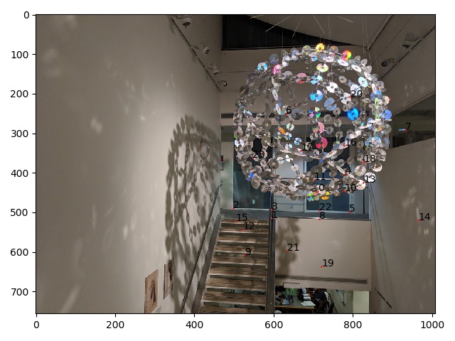
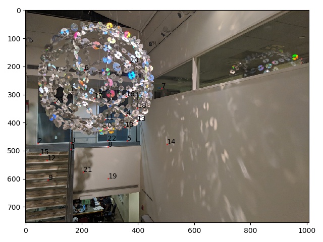
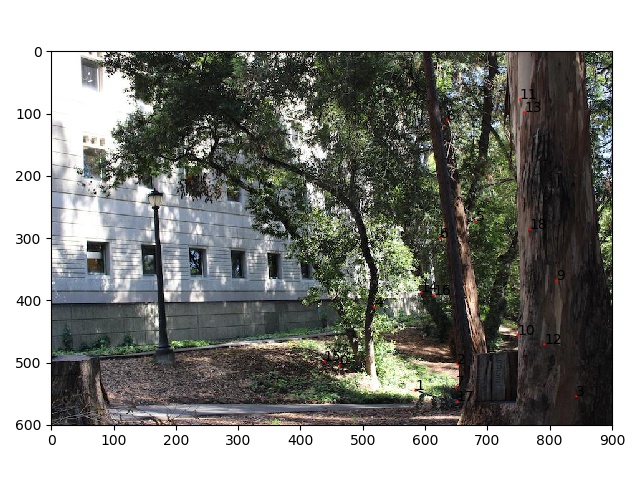
Example with manual warping:
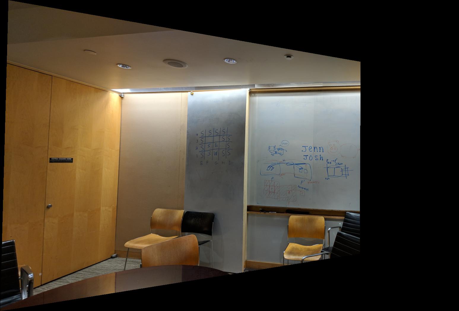
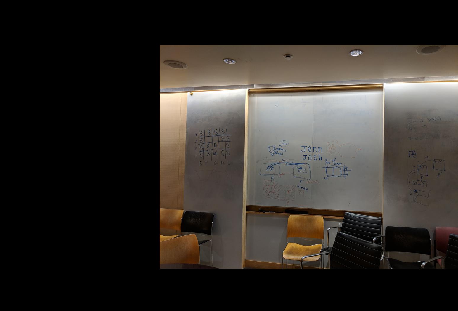
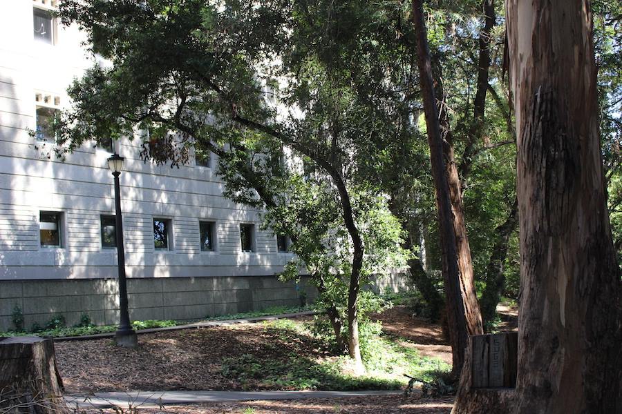
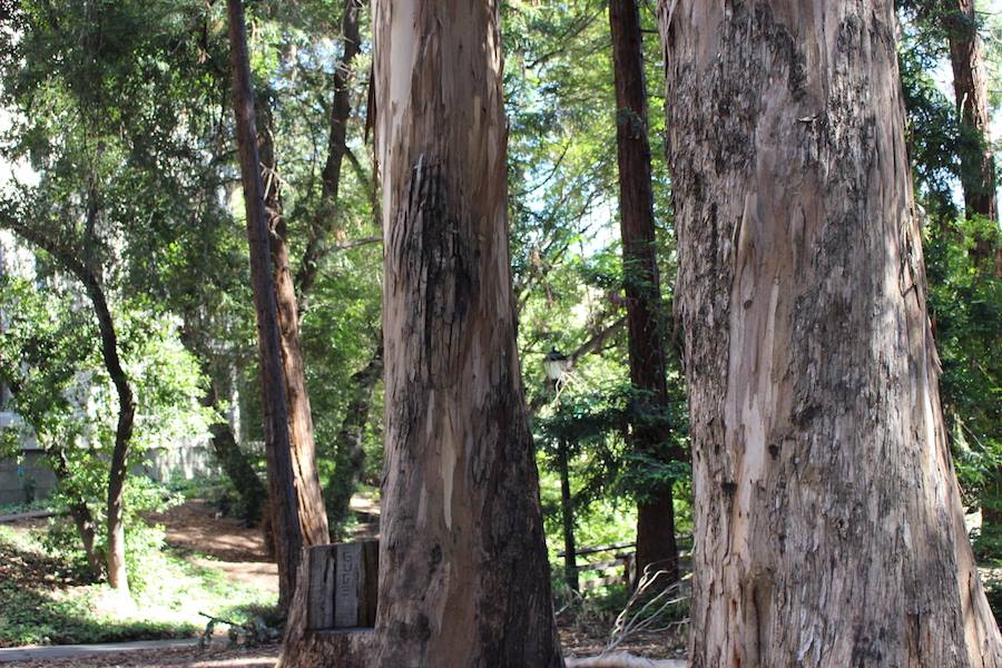
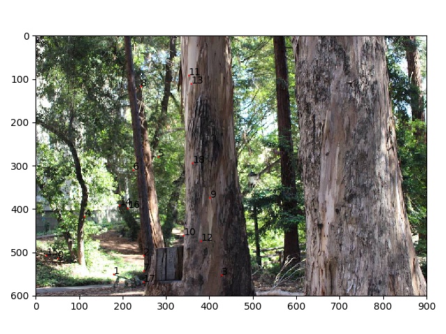
Original Images
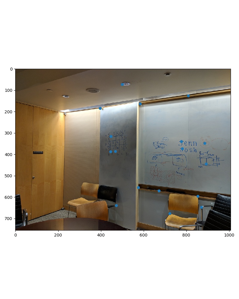
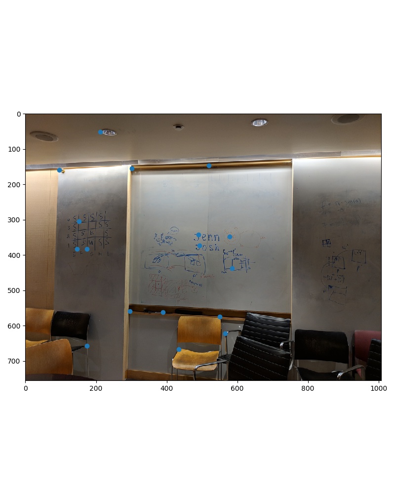
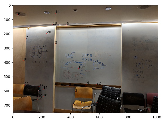
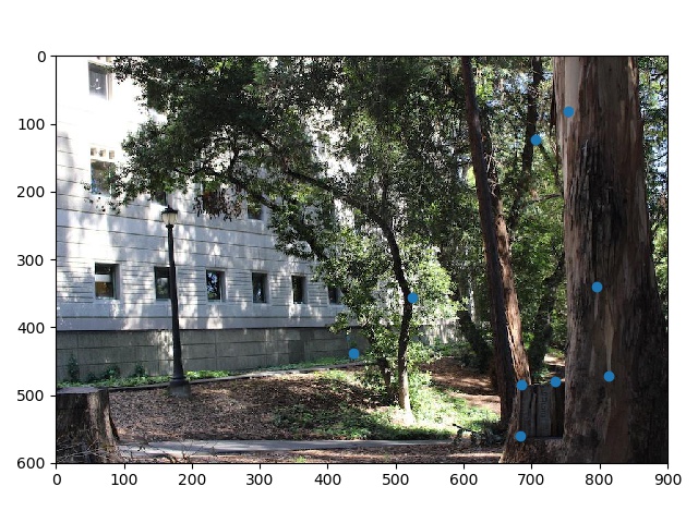
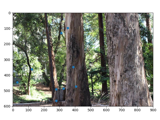
Manual Correspondences
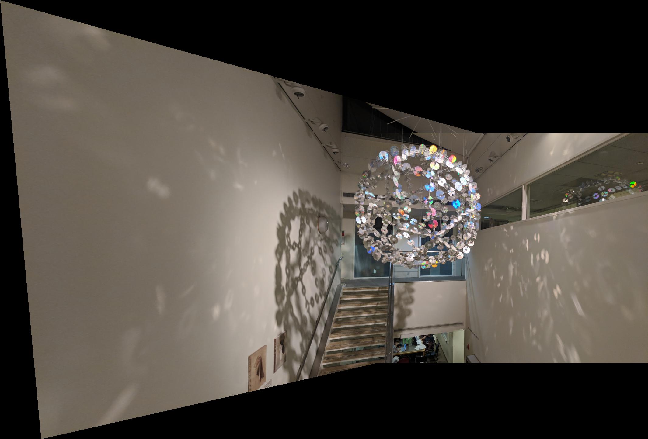
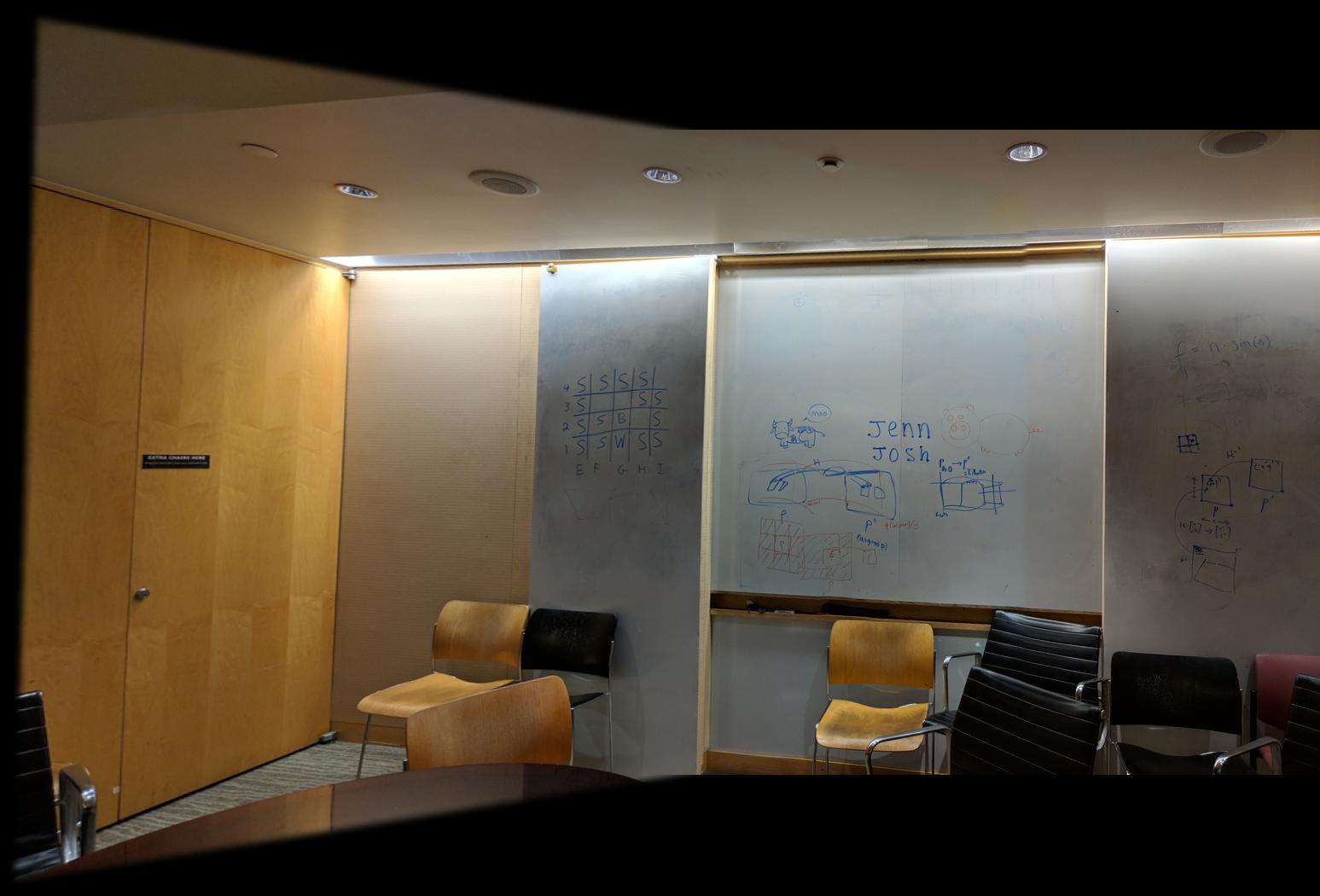
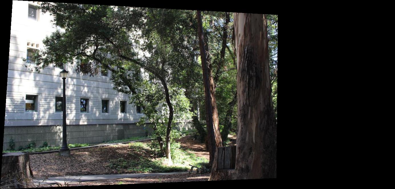
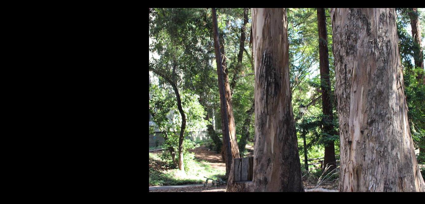
Warped and Translated
Blended
Blended by taking maximum for each pixel.
Part 2: Automatic Correspondences
We can improve our mosaic-maker by not requiring users to manually select correspondences but instead have our program automatically detect them.
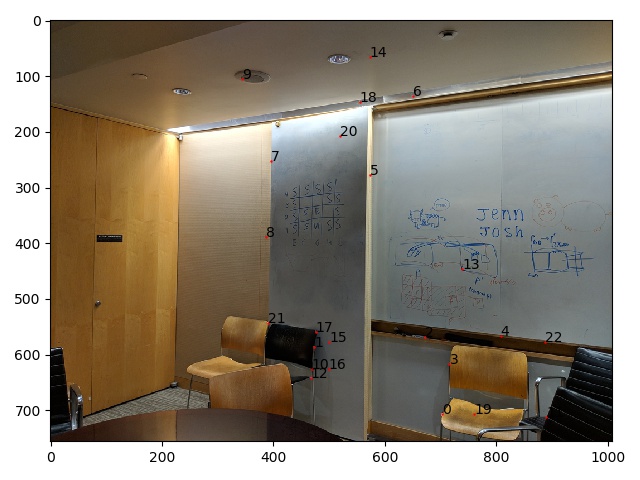
Interest Point Detection
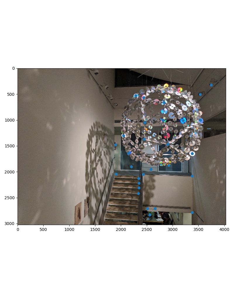
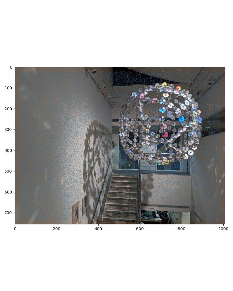
We detect potential interest points by using Harris Corner detection to find areas within the picture that are potential corners. This work by finding places where there are large derivitives in the x- and y- directions. This can result in hundreds or thousands of points so we nust refine.
Here are all the interest points detected in the image from above (marked in blue):
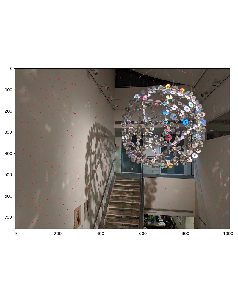
Adaptive Non-Maximal Suppression
We want to select interest points that we can use as correspondences between images which means we want many but we also want them spaced out. To do this, we use adaptive non-maximal suppression to suppress all but the top N points of interest (in this case 500 points). This is done by finding some radius r such that we only select points that have the maximal H value in their radius of size r. The H value is the heuristic from the Harris interest point detector, where higher values mean they are on stronger corners.
The way this is actually implemented is we select a scalar c, and find for each point x_i:

in other words, the distance to the closest neighbor of our point such that our point is greater than c times the neighbor's H value. We set c as .9. We then sort points by decreasing r_i and take the N (500) points with the largest r values.
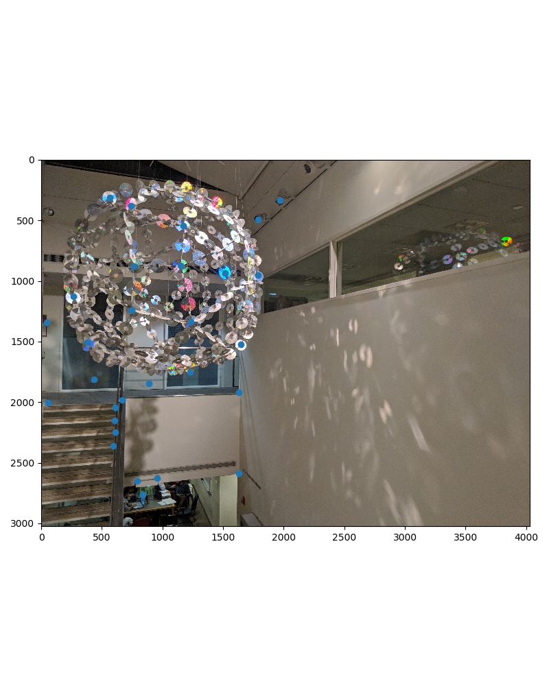
Here is our picture with the remaining points after supression:
Feature Descriptor Extraction
For each of the remaining chosen points of interest, we extract a feature from the image that will represent the point so we can use it for matching. In my case, I downscaled the image to a fifth of the size using Gaussian blurring in between, and then selected the 8x8 pixel patch around the point of interest to represent the point (representing the 40x40 patch around the point in the original size image). We then all convert them to be zero-meaned and having an SD of 1.
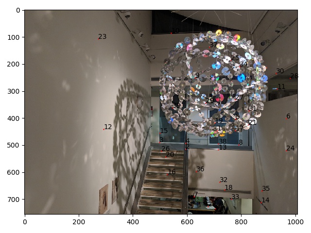
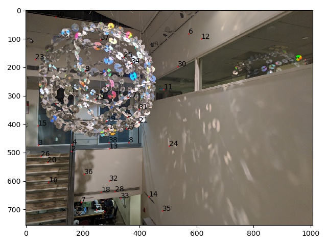
Feature Matching
For the two images, we then compute the SSD between each of image 1's points' features and image 2's points' features. For each point in image 1, we find its best match (smallest SSD) from image 2 as well as its second best match. We compute SSD(best)/SSD(2nd best), and if this is greater than a threshold (we set it as .6), then we say that the point in image 1 corresponds with the best matches point in image 2. Otherwise we just throw away point 1 and don't use it.
Here is our images' points after feature matching.
Finding a Homography with RANSAC
Finally we need to find the homography that will transform image 1 into being properly aligned into image 2. We can use our homography solver from part 1 to do this, but it is not enough to use our points from feature matching because one inaccuracy or mismatch in correspondences can lead to poor fitting of the homography if large enough.
To handle this, we use RANSAC which is done as follows:
- Select 4 points from image 1 at random.
- Compute the homography from those 4 points to their corresponding points in image 2.
- See how many inliers there are. Inliers are all potential correpondence points that, when transformed with our homography, are within t pixels away from their actual correspondence detected from earlier. We set t to 5.
- If there are more inliers than our current best homography, save this set of inliers.
- Repeat 1-4, many times (in this case 50).
- Calculate our homography using the set of inlier points from the best homography.
After running RANSAC, we removed some outliers and got the following points.
Results
With these automatically calculated correpsondence points and homography, we use part 1 to stitch our images together. We get the following:
Final Results
Soda 7th Floor
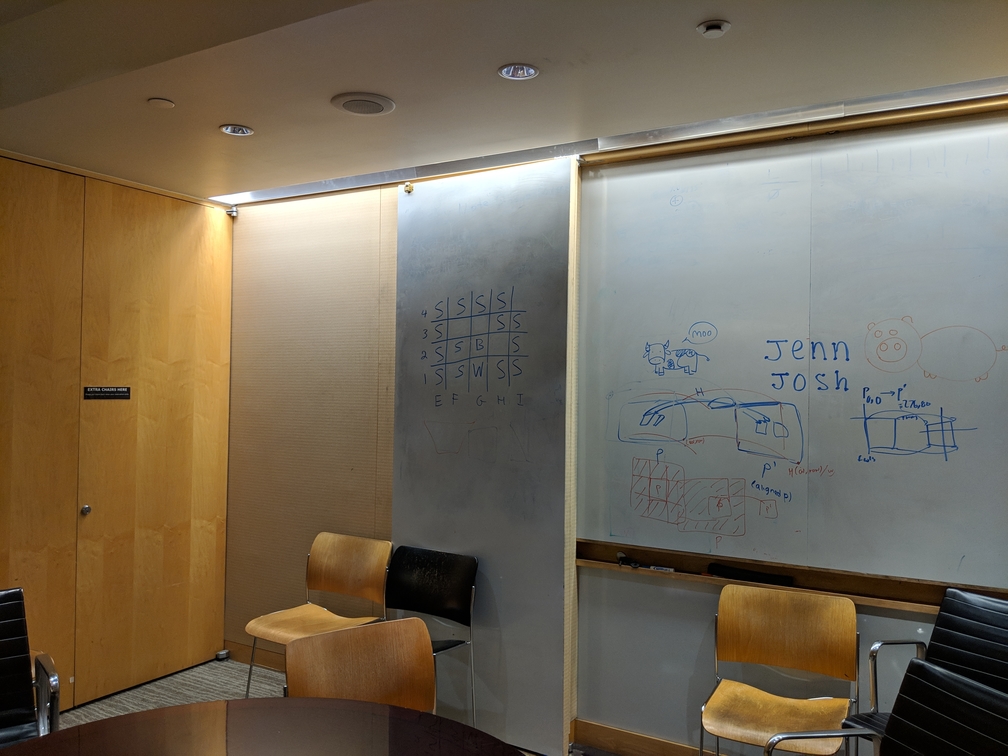
Original Images
Manual Correspondences
Automatic Correspondences
Warped and Translated (from Manual)
Blended
Blended by taking maximum for each pixel.
Manual:
Automatic:
606 Soda
Original Images
Manual Correspondences
Automatic Correspondences
Warped and Translated (from Manual)
Blended
Blended by taking maximum for each pixel.
Manual:
Automatic:

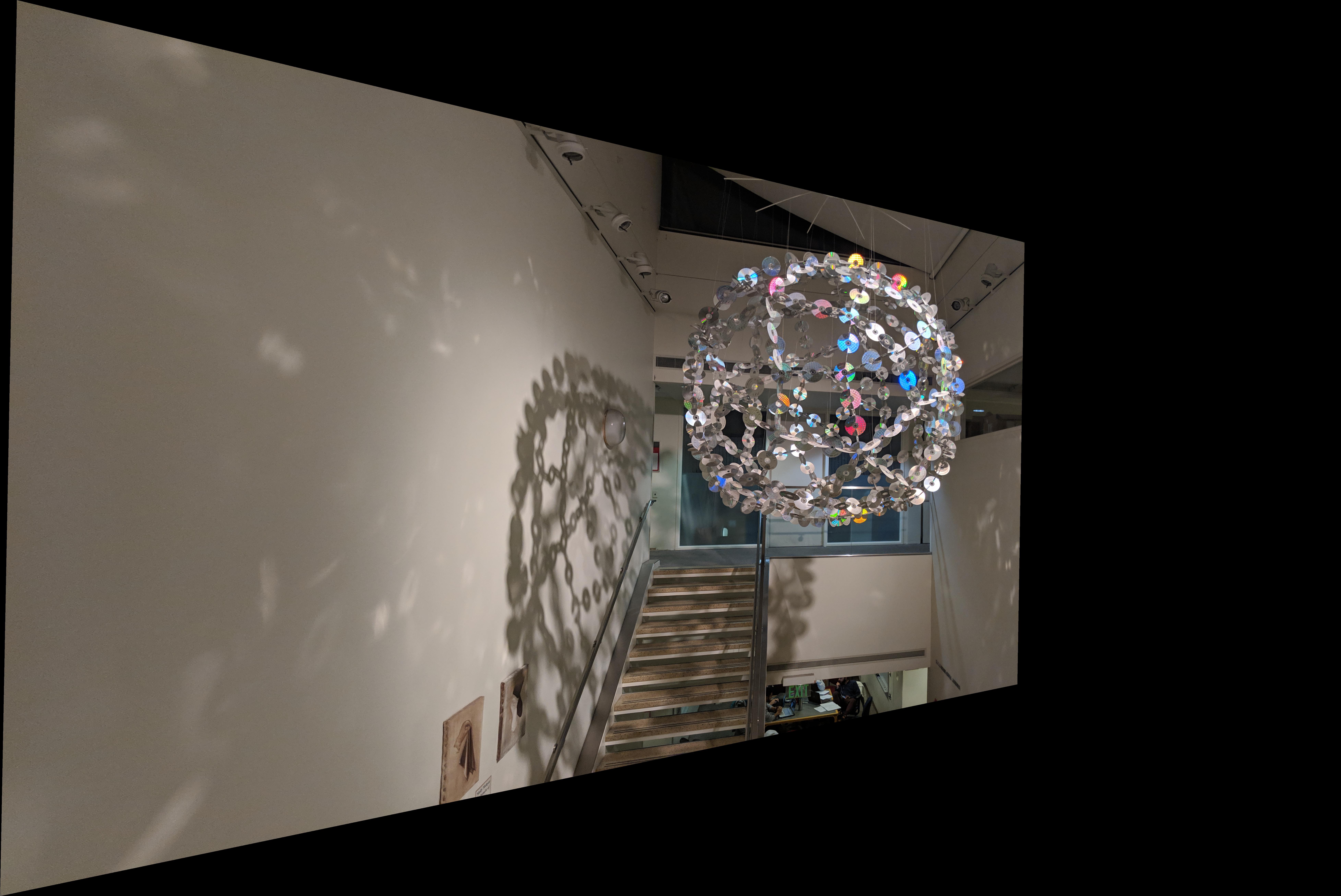
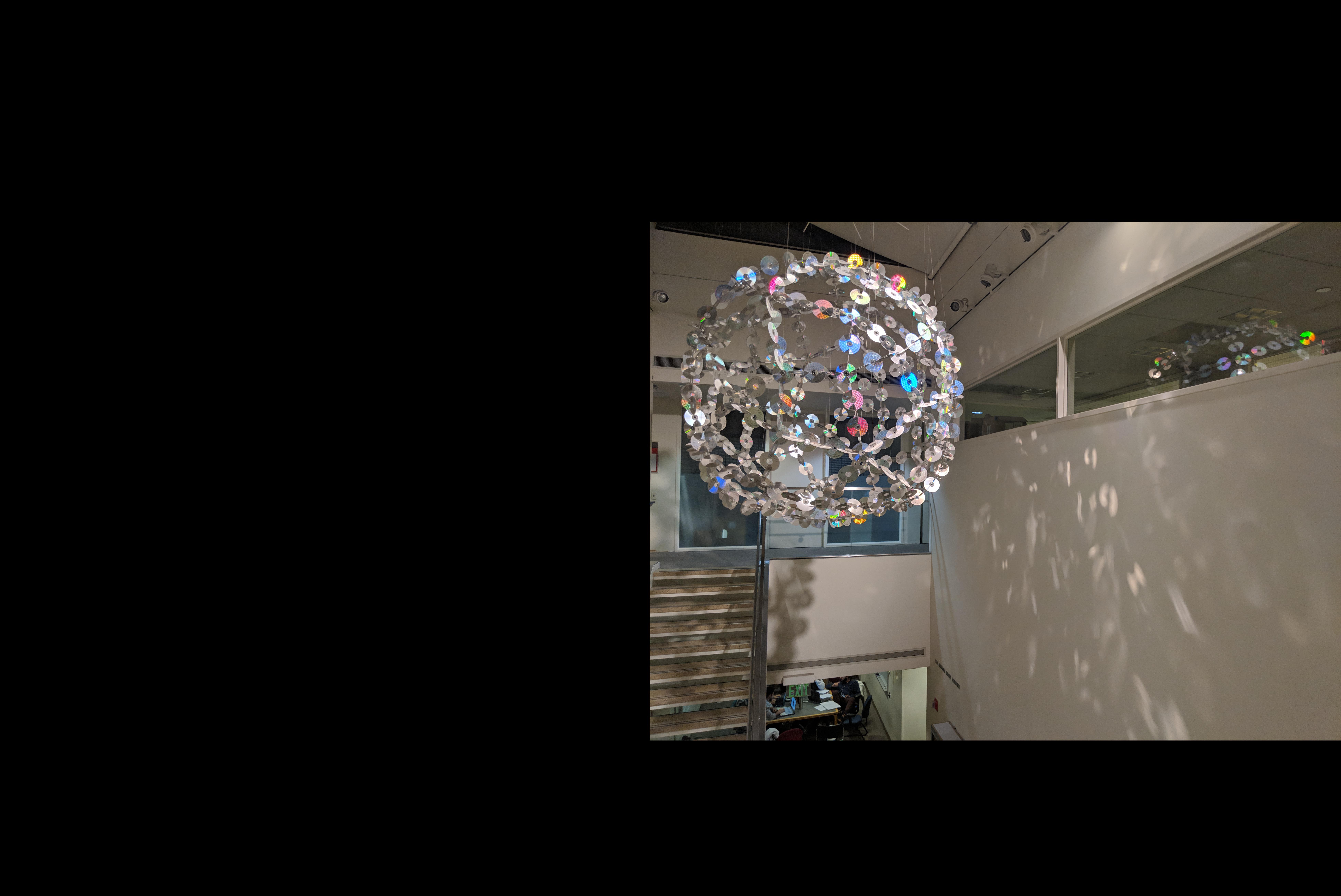
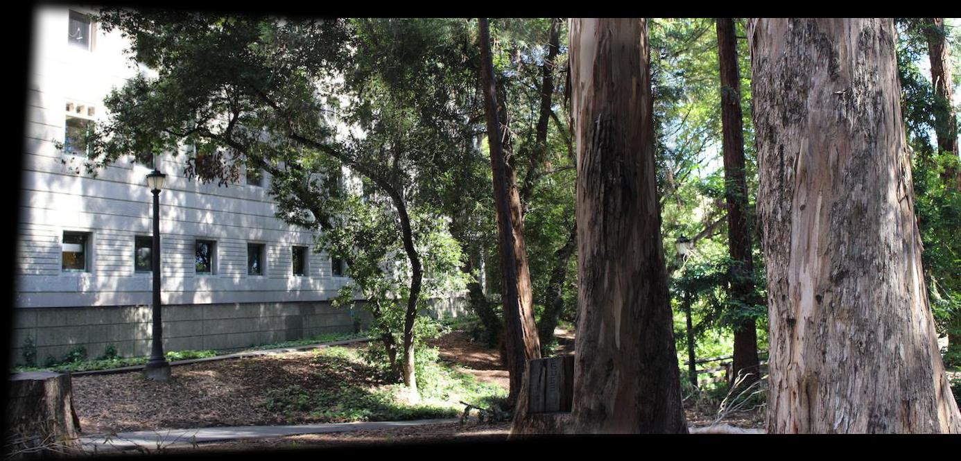
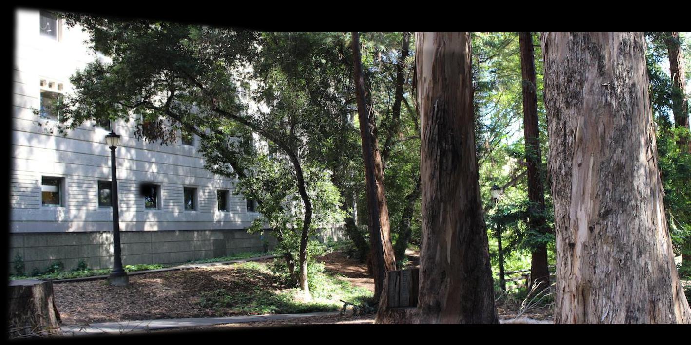
West Campus
Original Images
Manual Correspondences
Automatic Correspondences
Warped and Translated (from Manual)
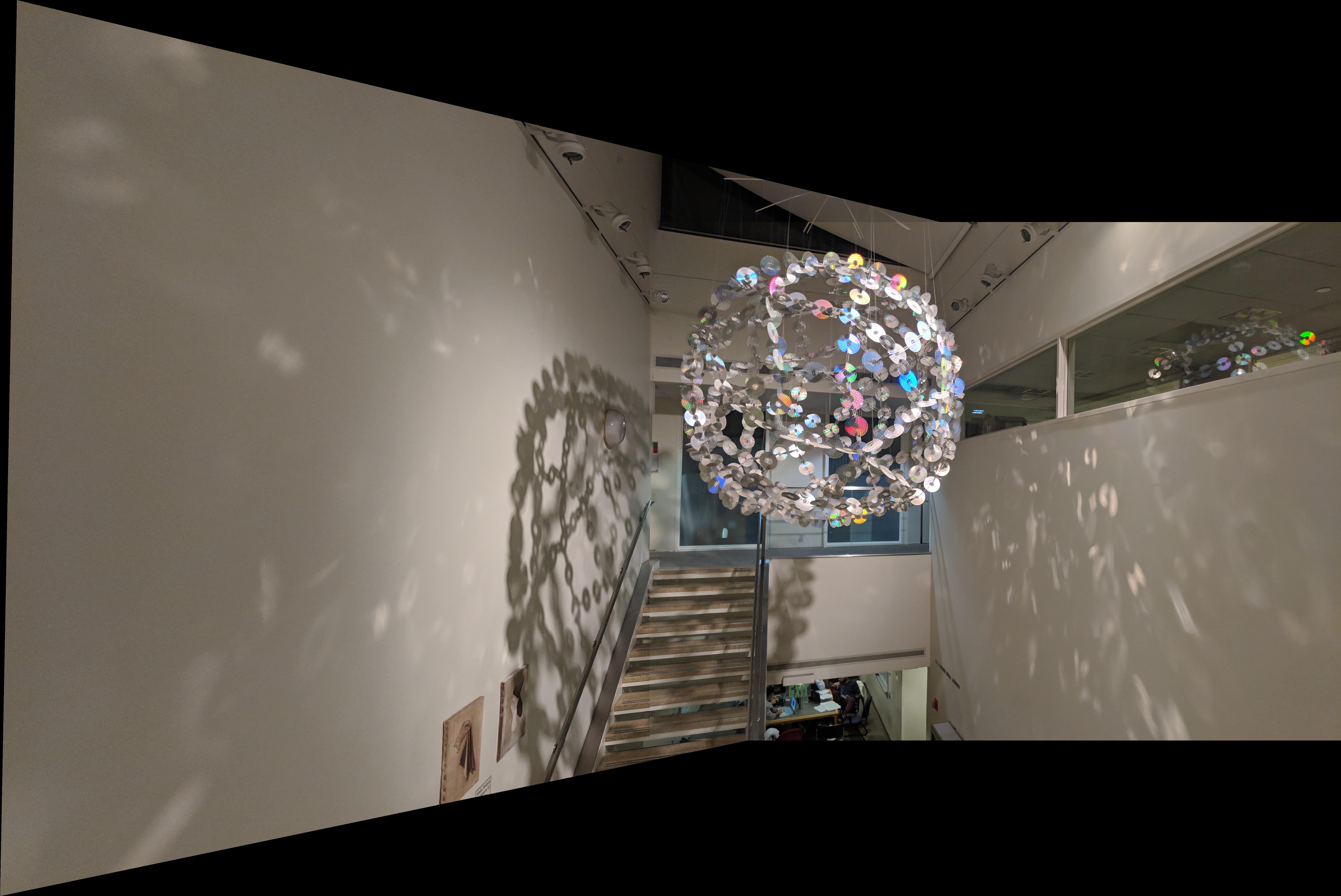
Blended
Blended by taking maximum for each pixel.
Manual:
Automatic:
What I Learned
I learned that taking good pictures is really important for mosaicing! Having consistent lighting is important so that stitching takes minimal work to not appear to have seams. In addition, not translating the camera while taking pictures is important as well to avoid inconsistent panoramas. Having more correspondence points is also useful so that human error in selecting them is minimized (i.e. the final homography and translating/stitching of the image involves solving a least-squares equation or taking an average and so human error is averaged out).
In the second part of the project, the coolest part was implementinc RANSAC. It showed how a median / mode can be a better estimator than the mean. If we took all the points we received from matching and just computed our homography off of that, it's similar to taking the mean of points - one outlier can give a completely wrong transformation. However, if we take a median/mode, i.e. only take the points that are consistent with most of the rest, then we can resist outliers and obtain an accurate homography.