Image Rectification
In order to rectify an image, I first recover its homography (i.e., the matrix with eight degrees of freedom and a scaling parameter that projectively tranforms points in one image to corresponding ones) using a least-squares approximation. I then warp that image using that homography to a plane that is frontally parallel (e.g., the corners of the original image).
Rectifications
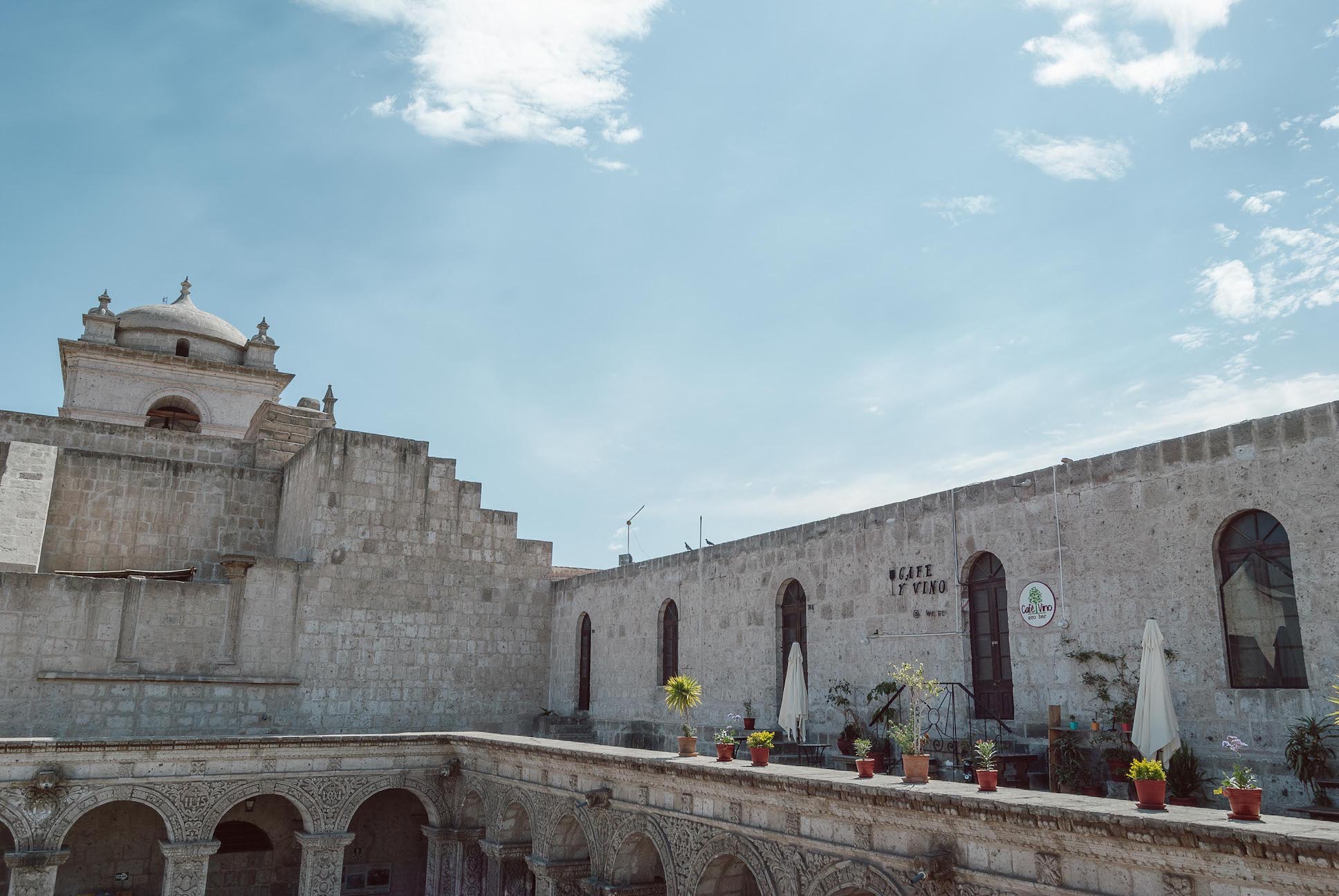
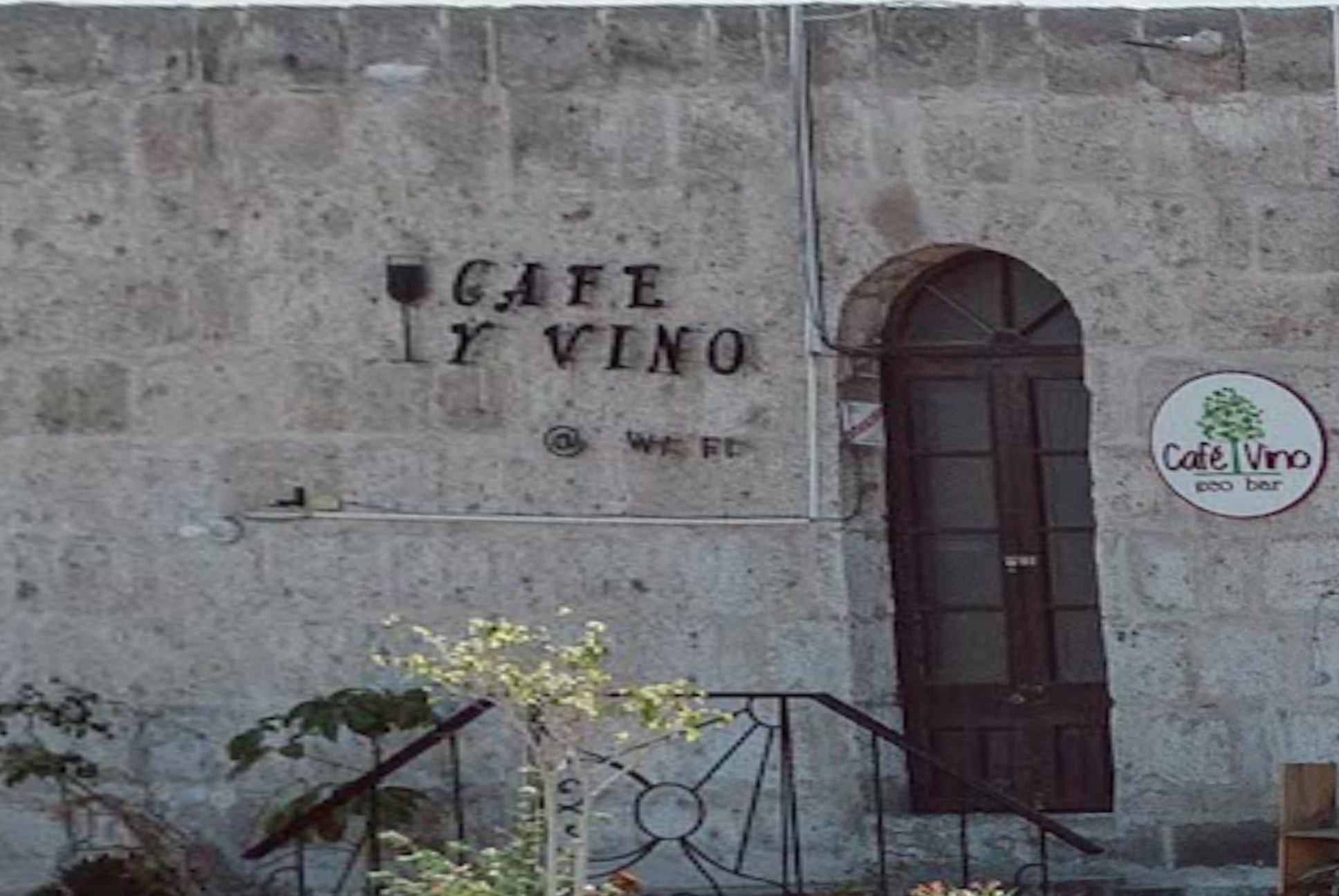
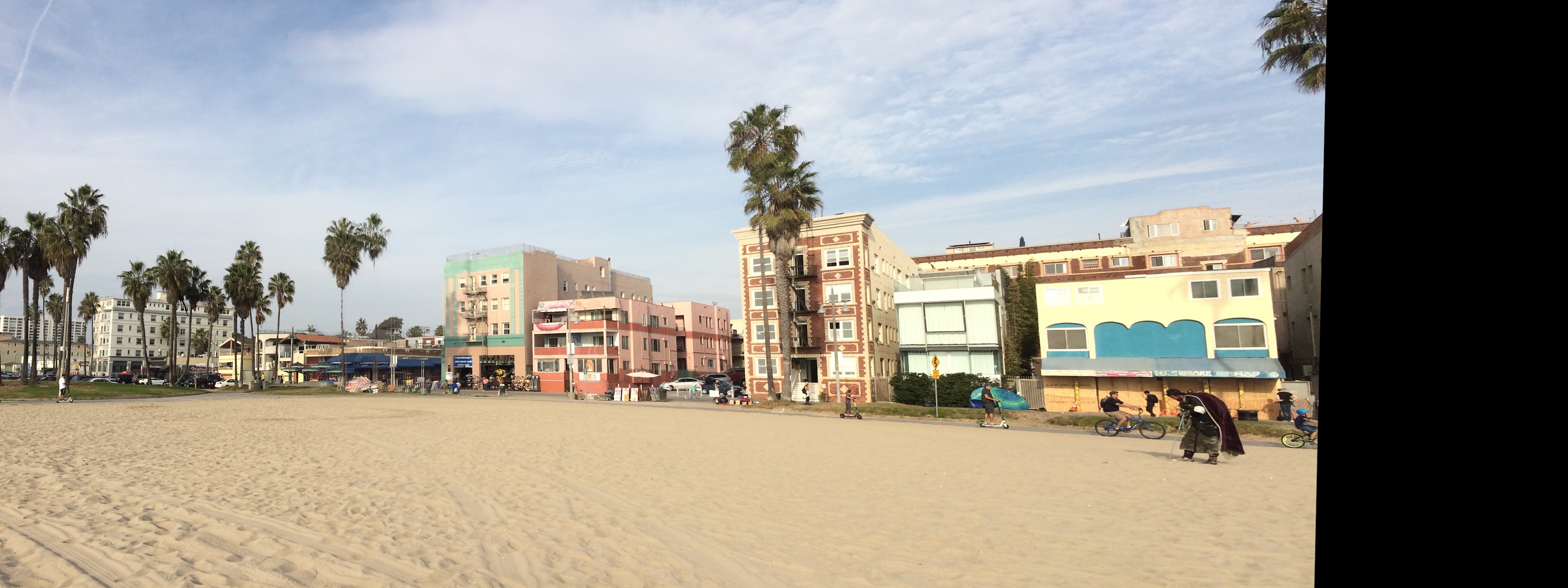
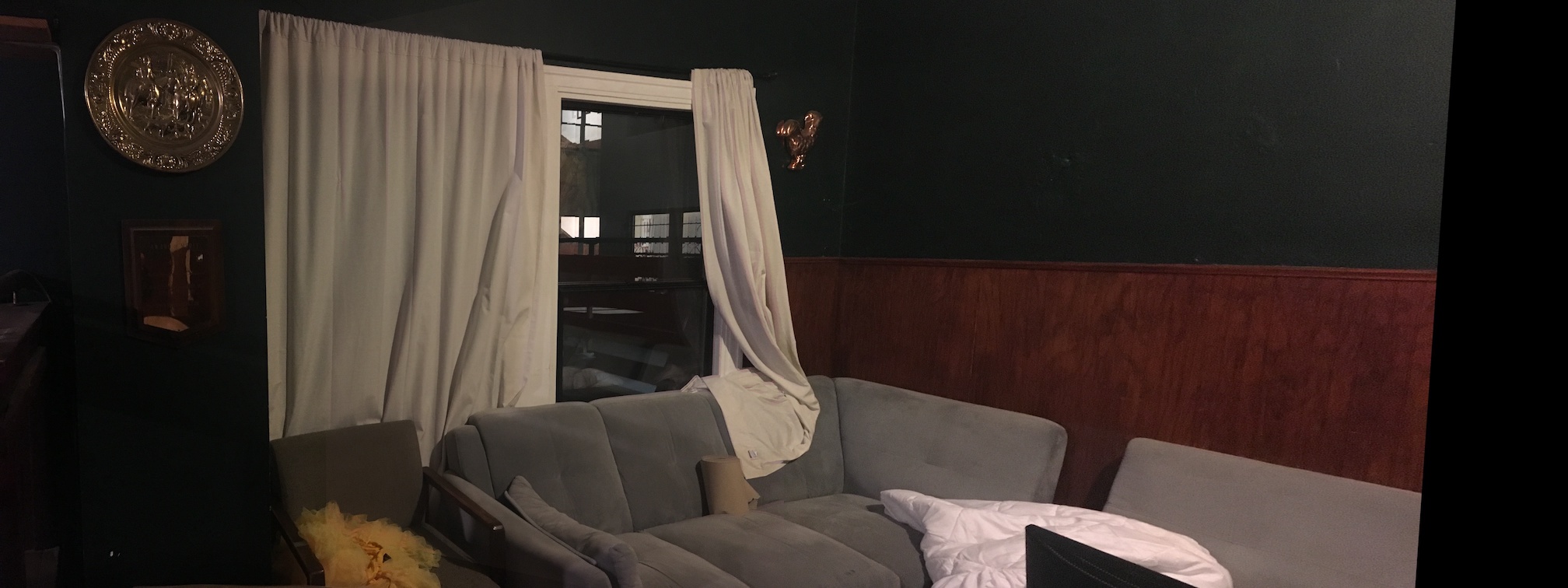
 Original
|
 Rectification with Custom Corners
|
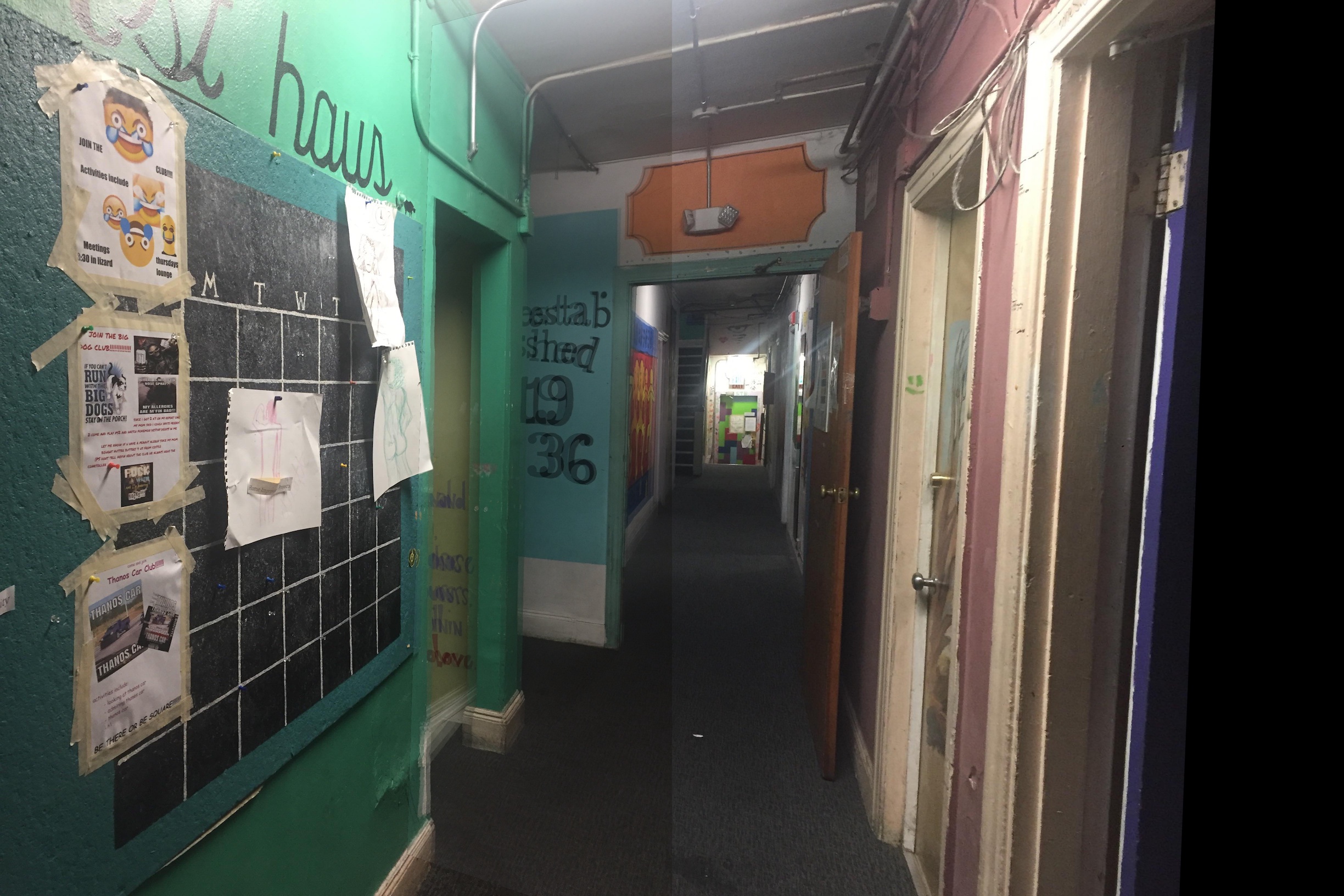
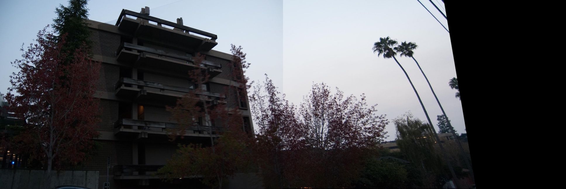
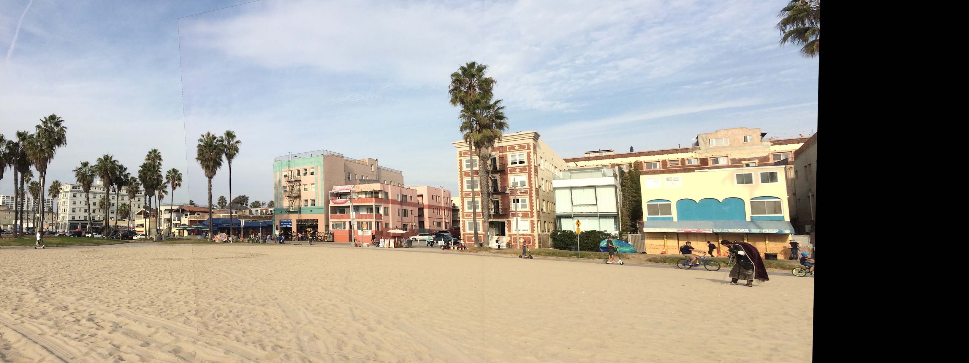
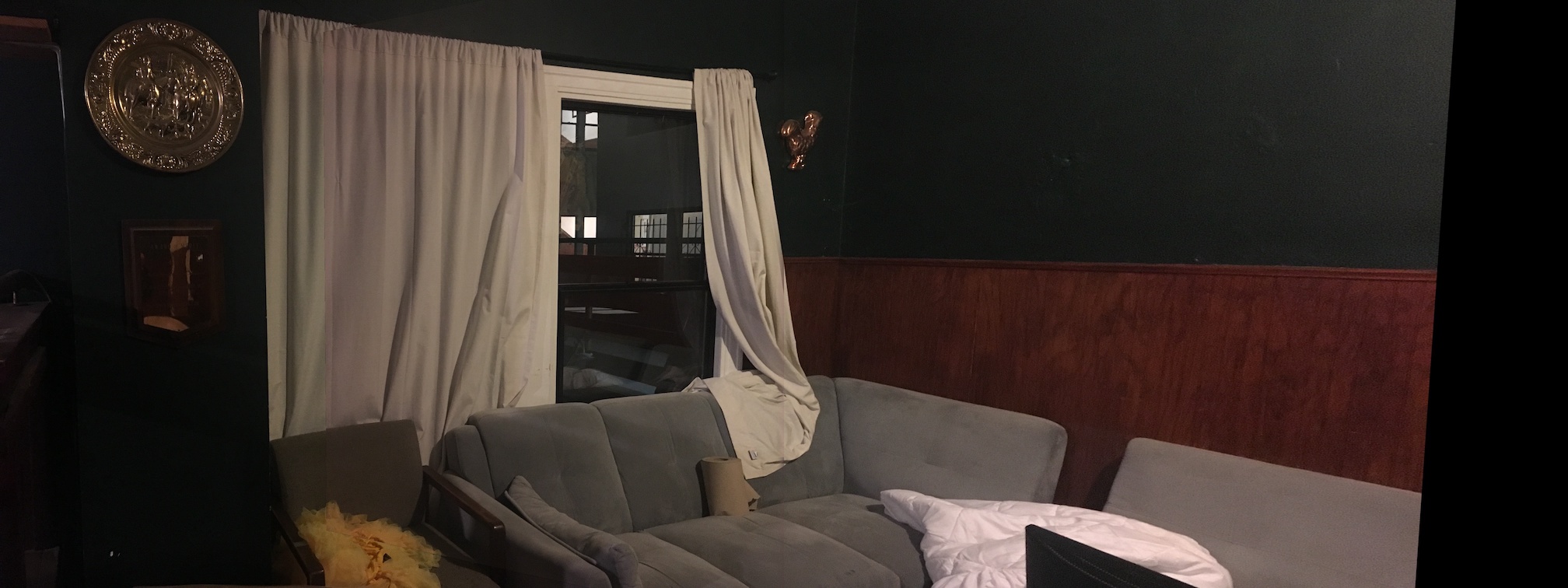
 Rectification with Canvas Corners
|
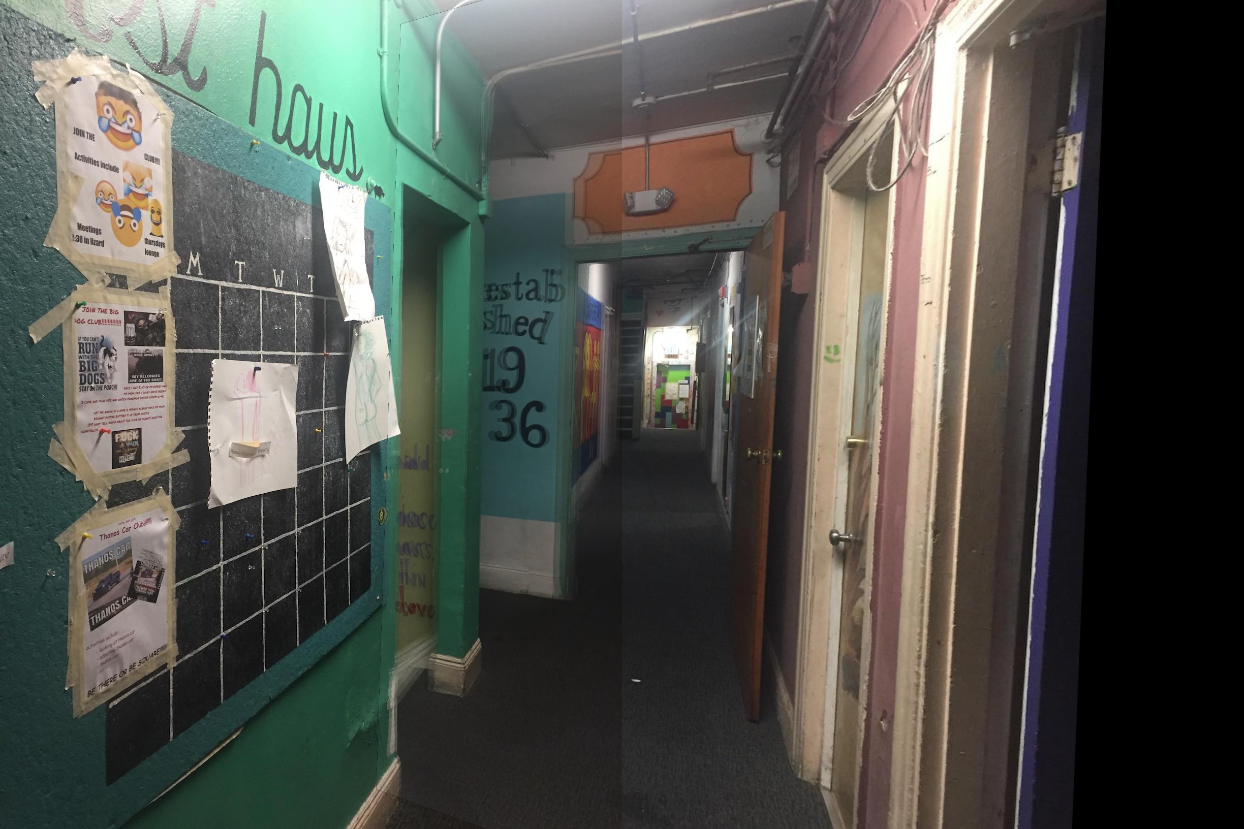
 Original
|
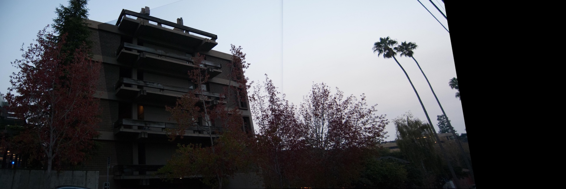
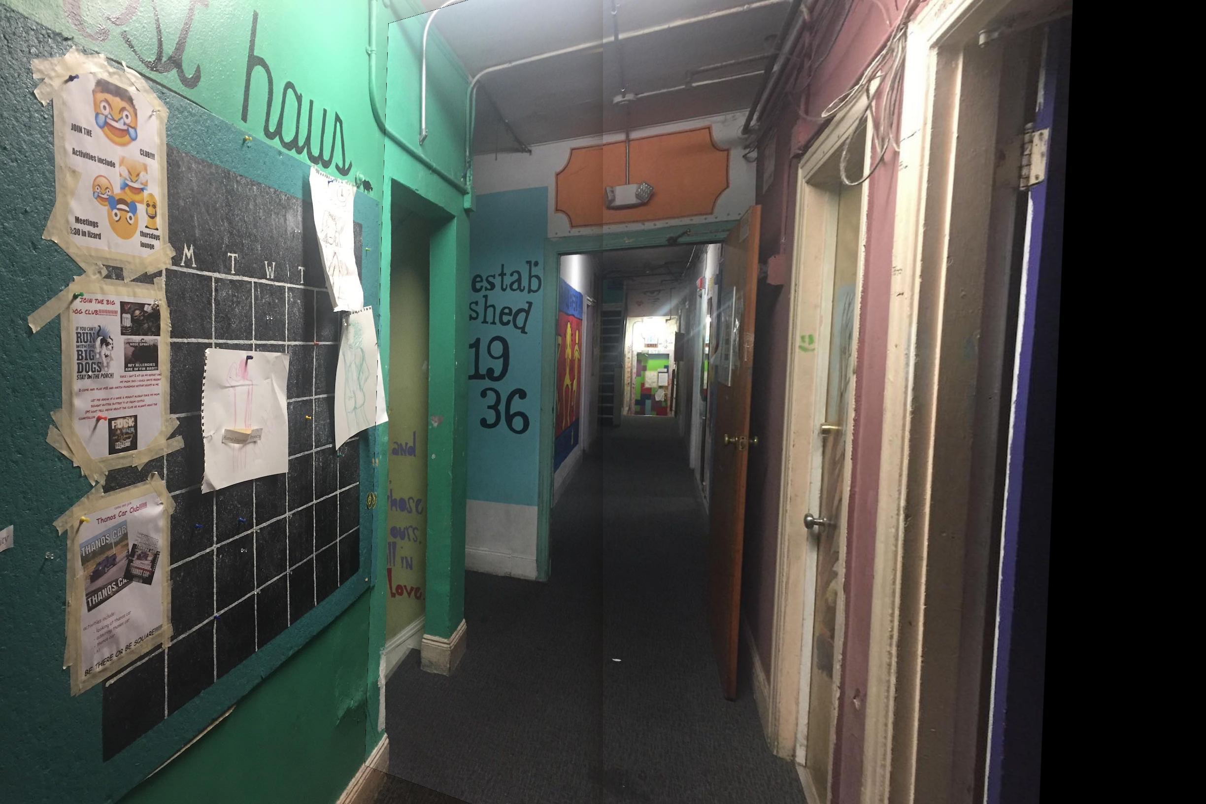
 Rectification with Canvas Corners
|
Blending Images into a Mosaic
Blending images starts with the same logic. I actually select eight correspondences to produce an overdetermined system, and I warp the second image to the first in order to make blending the images easier. I try multiple techniques for blending: weighted averaging, maximim pixel value, and Laplacian blending using two levels.
Mosaics
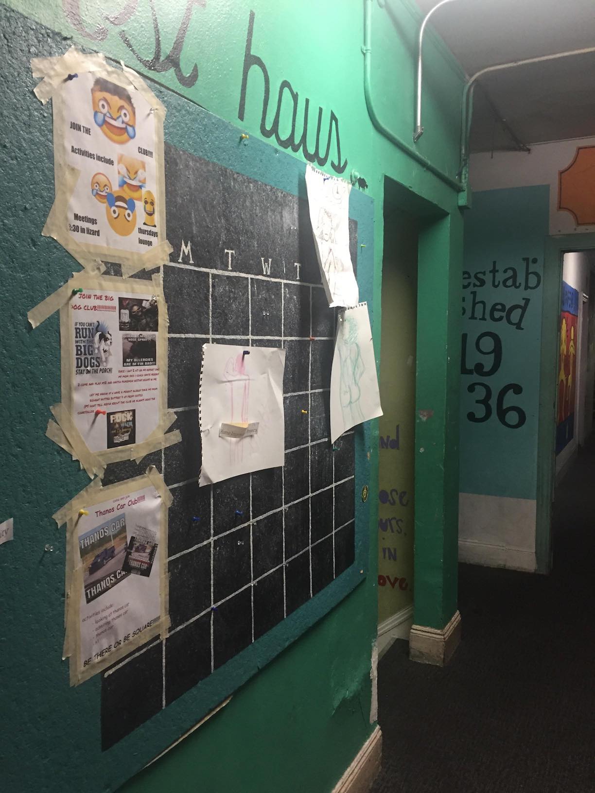 Image 1
|
|
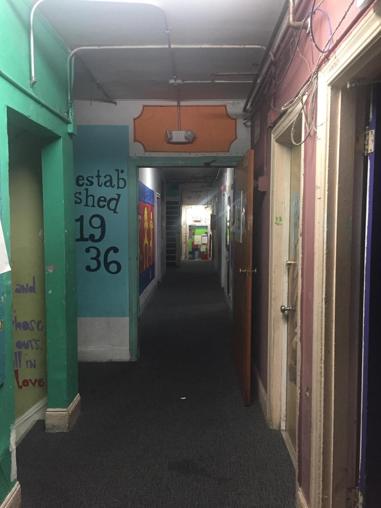 Image 2
|
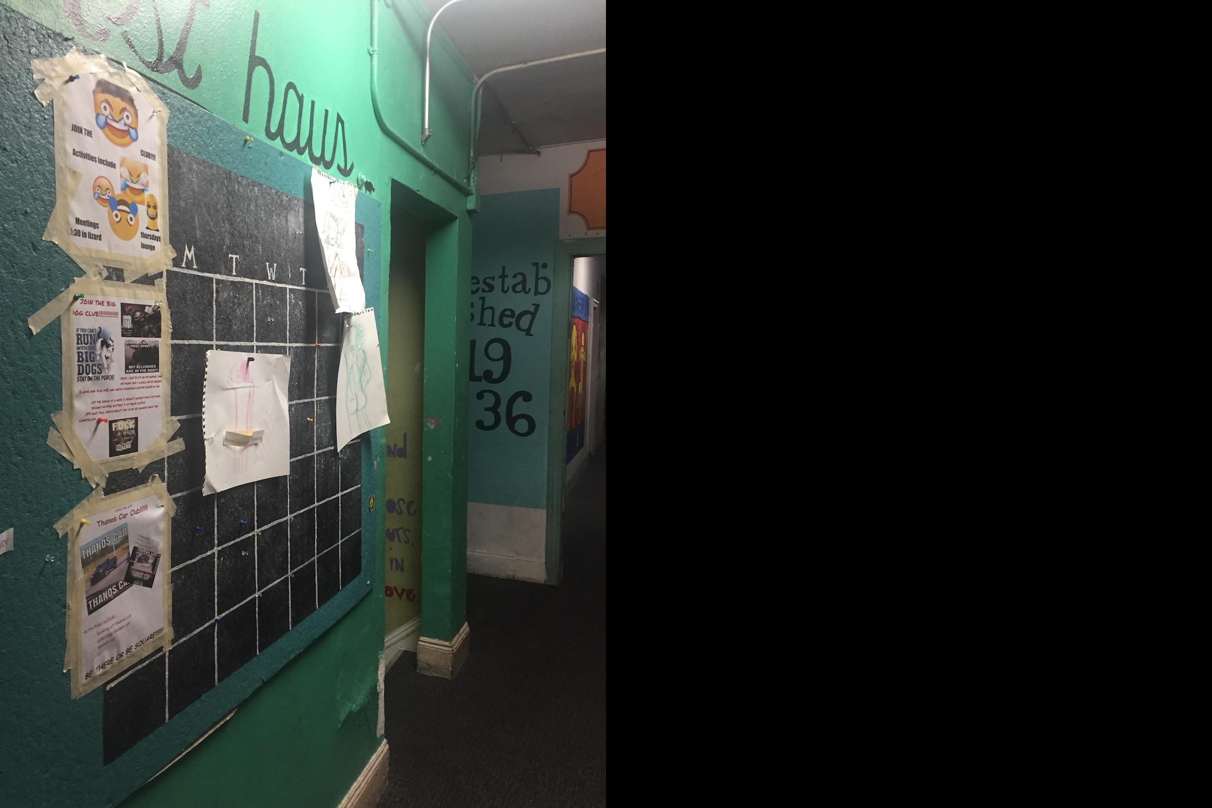 Image 1 Padded
|
|
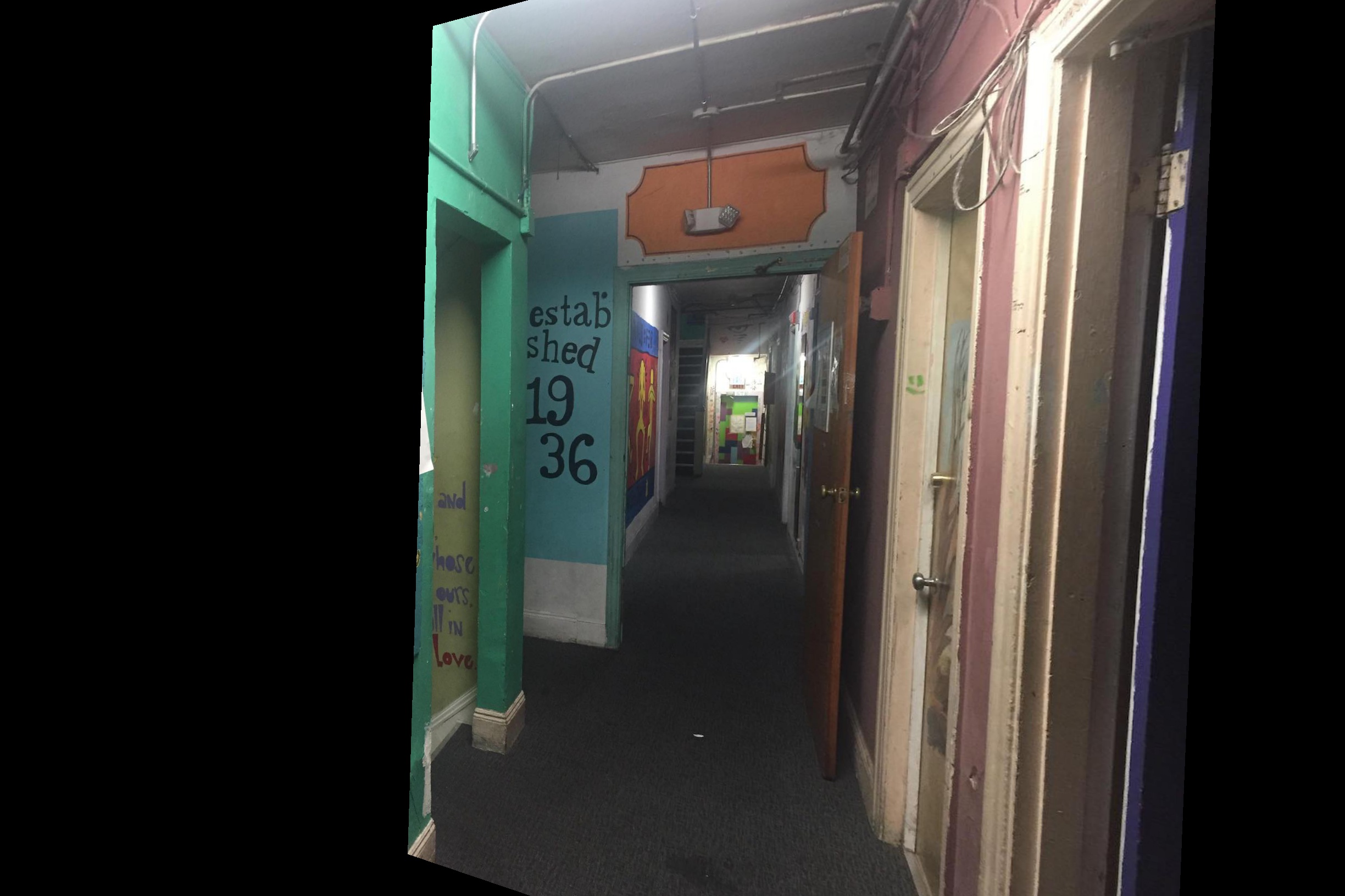 Image 2 Rectified
|
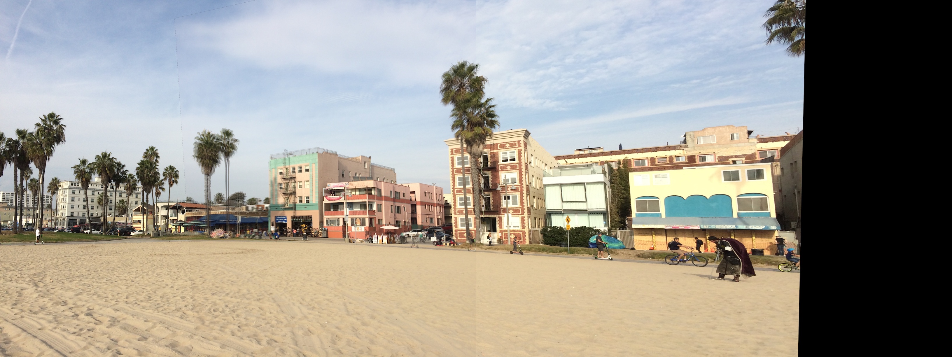
 Average Blending
|
 Max Blending
|
 Laplacian Blending
|
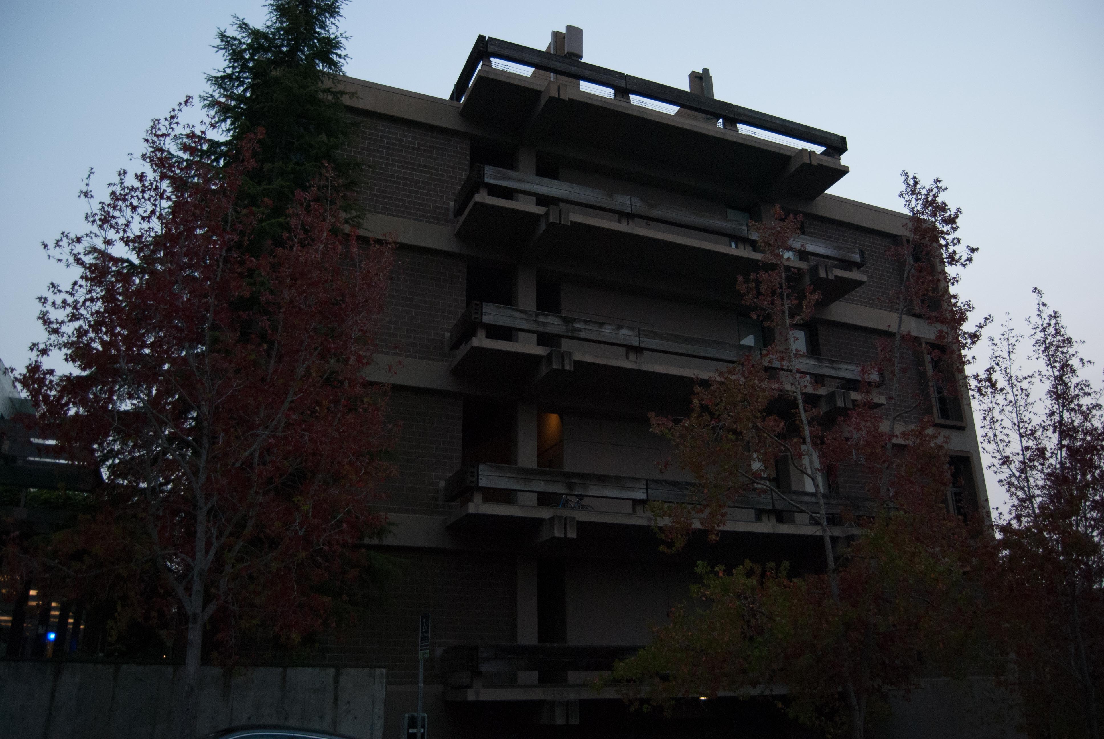 Image 1
|
|
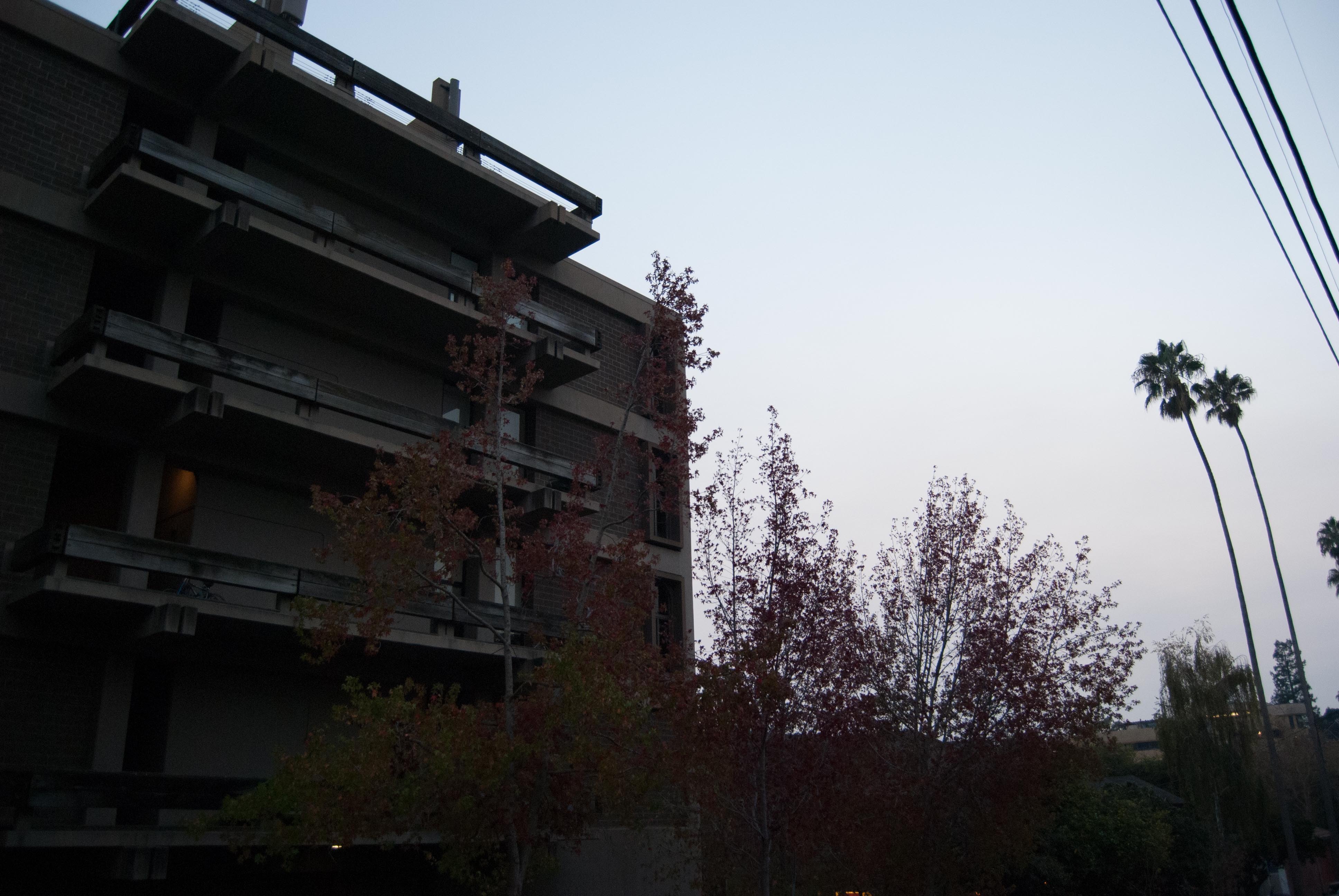 Image 2
|
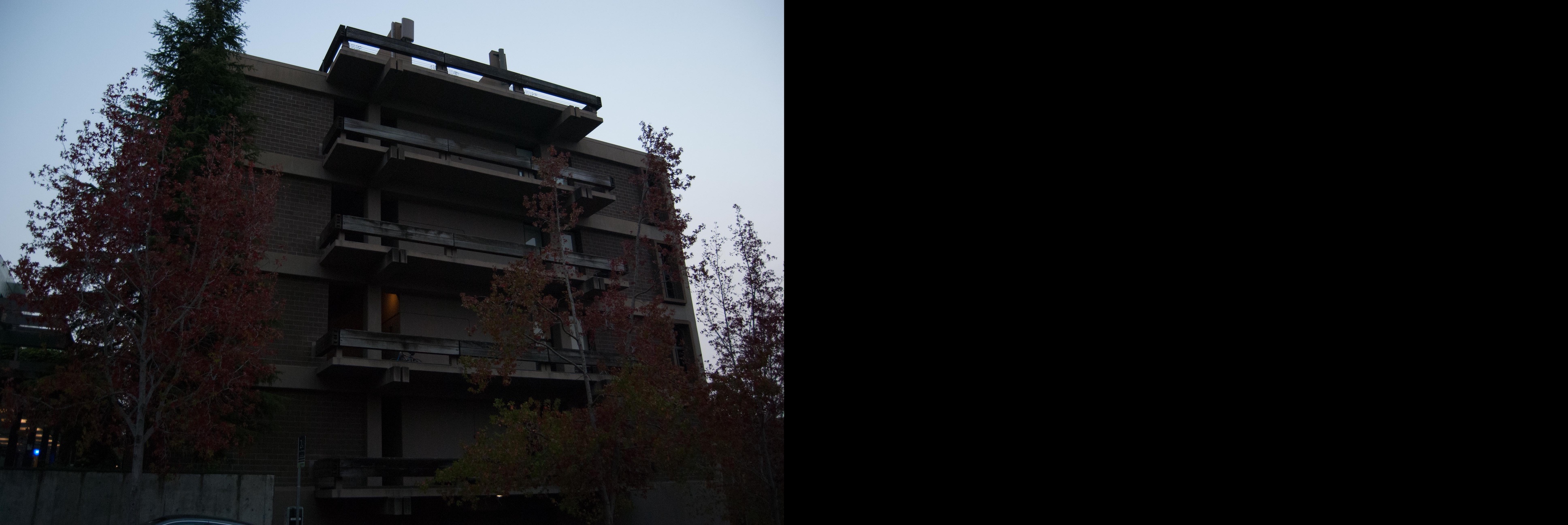 Image 1 Padded
|
|
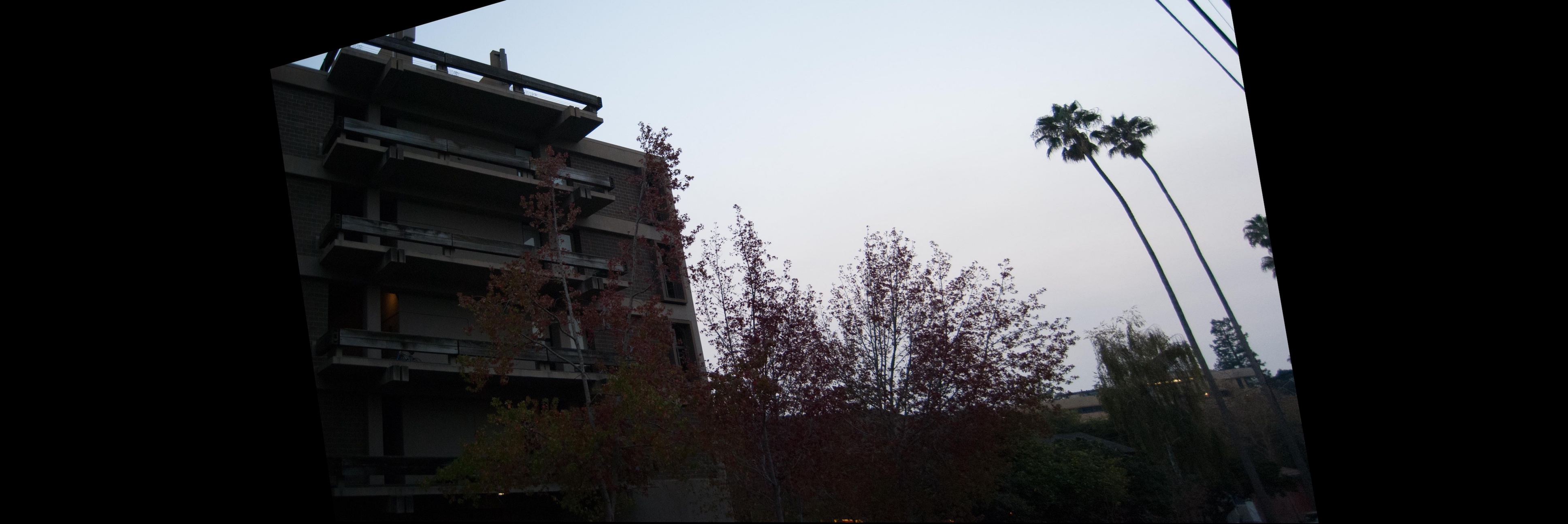 Image 2 Rectified
|
 Average Blending
|
 Max Blending
|
 Laplacian Blending
|
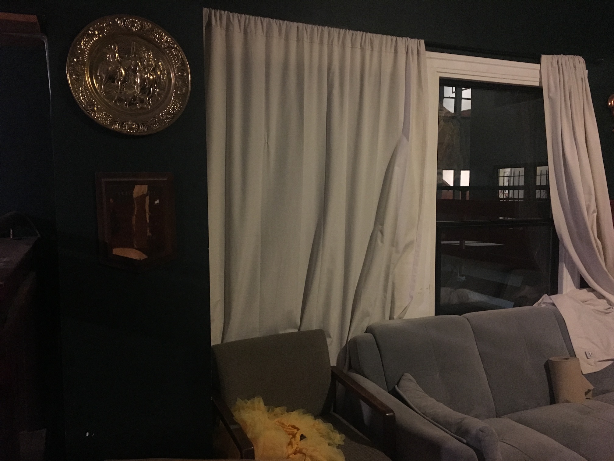 Image 1
|
|
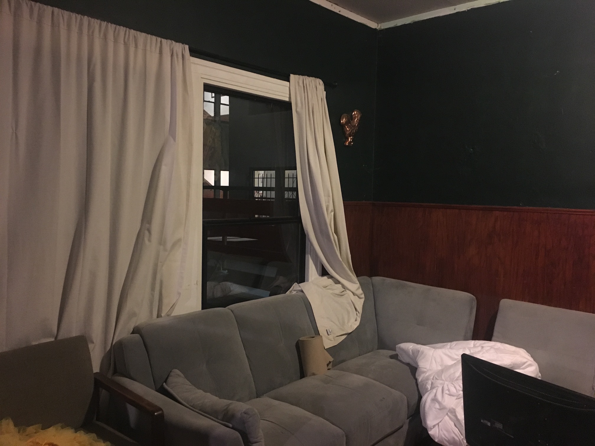 Image 2
|
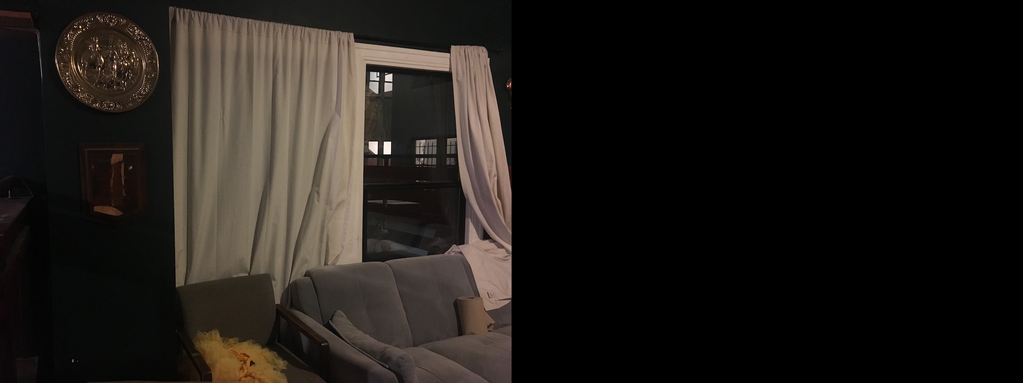 Image 1 Padded
|
|
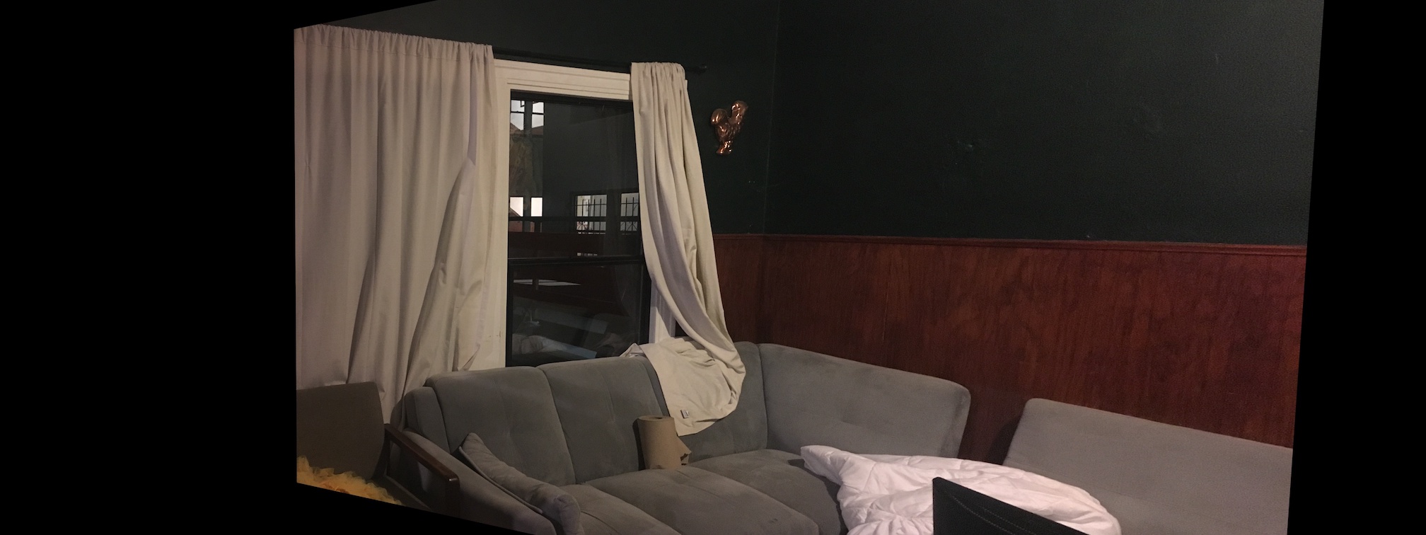 Image 2 Rectified
|
 Average Blending
|
 Max Blending
|
 Laplacian Blending
|
Harris Interest Point Detection
Manually selecting corresponding points in both images is tedious and not so accurate. I therefore implement the strategy outlined in Multi-Image Matching Using Multi-Scale Oriented Patches to automate the process. I start by detecting interest points using a single-scale variant of a Harris Corner Detector using scikit-image's feature.corner_harris function.
Harris Corners with min_distance=20
 3893 Points
|
 3815 Points
|
Adaptive Non-Maximal Suppression
I restrict the number of interest points in each photo to 500 using ANMS to select only corners that are maxima within an appropriate radius.
ANMS Corners with c_robust=.9
 500 Points
|
 500 Points
|
Extracting Feature Descriptors
In order to match corresponding corners between the two images, I extract a description of the local image structure by storing 40x40 windows downsampled to 8x8 and bias/gain-normalized.
Matching Features
I now find pairs of features that look similar by computing the distances between the descriptors for the corners in both images and making matches if the ratio between the two nearest neighbors of each feature in the first image is below a certain threshold.
Feature Matches with threshold=.33
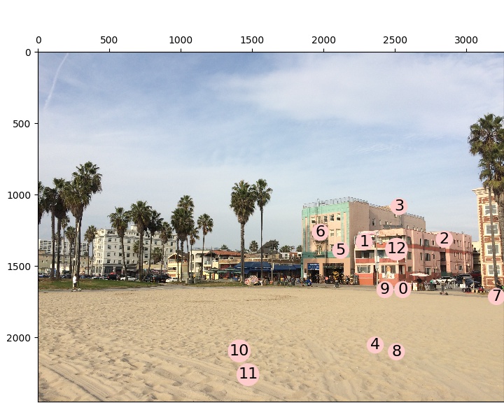 Image 1 Matches
|
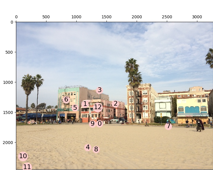 Image 2 Matches
|
Note that point 7 is a bad match since the person moves between images. This is addressed in the following section.
Random Sample Consensus
To get rid of bad matches, I implement four-point RANSAC by selecting four feature pairs at random, computing the exact homography, and then computing inliers. I repeat this process many times and keep the largest set of inliers generated and then compute the least-squares homography on that set.
Feature Matches after RANSAC with epsilon=.75
 Image 1 Matches
|
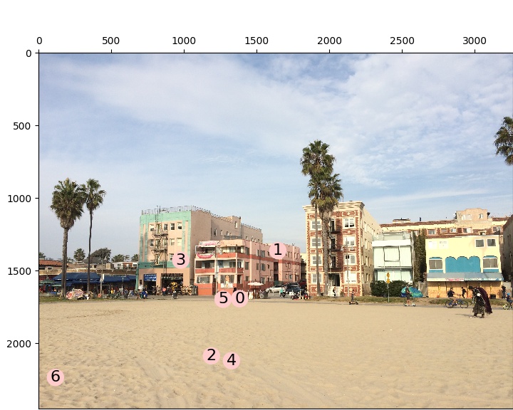 Image 2 Matches
|
Auto-Stitched Mosaics
 Image 1
|
|
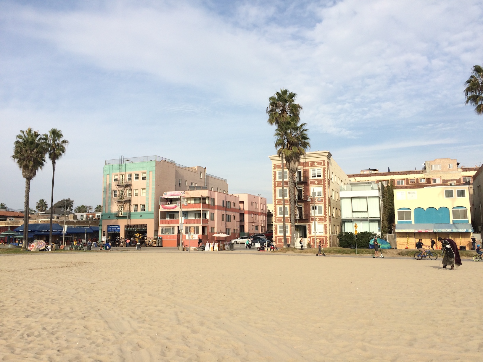 Image 2
|
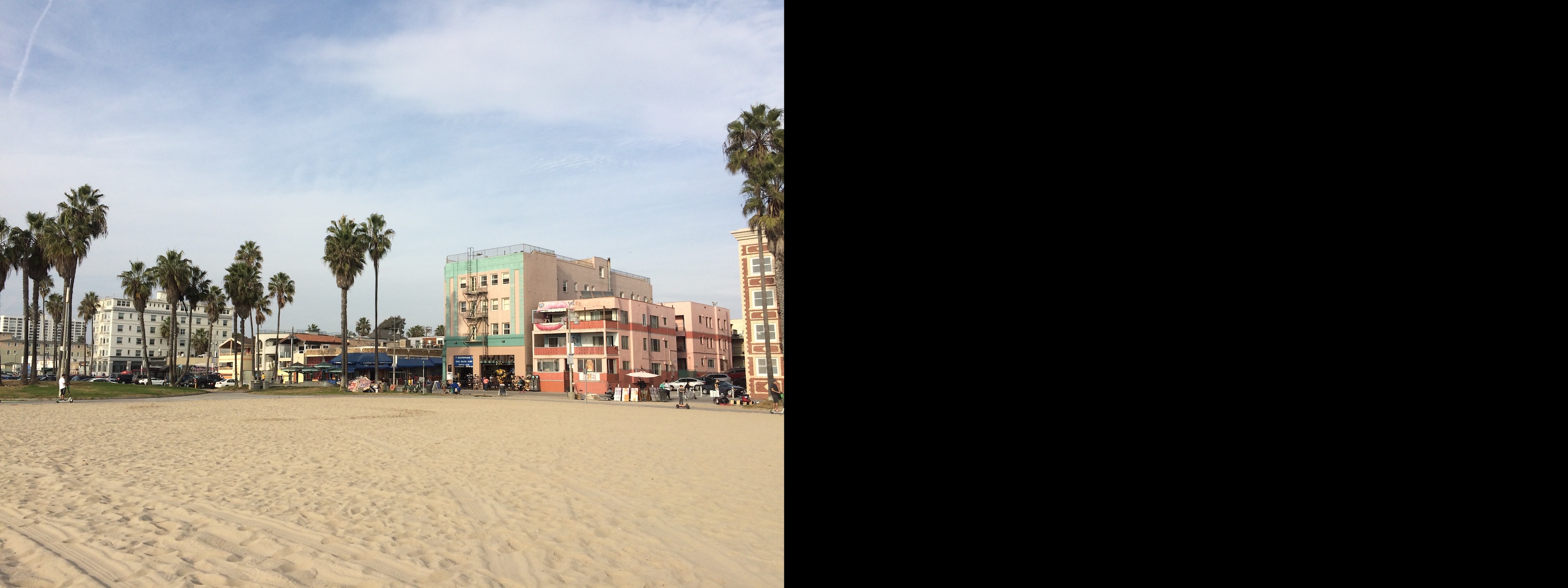 Image 1 Padded
|
|
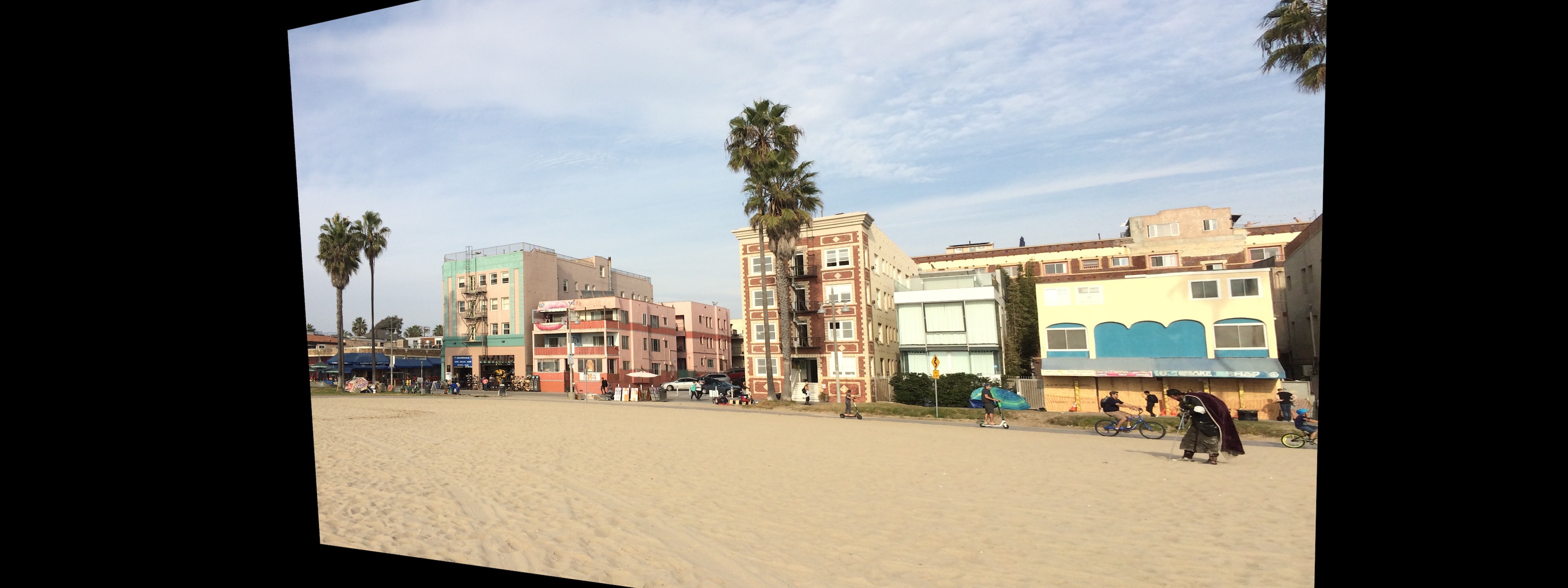 Image 2 Rectified
|
 Average Blending
|
 Max Blending
|
 Laplacian Blending
|
 Average Blending
|
 Max Blending
|
 Laplacian Blending
|
 Average Blending
|
 Max Blending
|
 Laplacian Blending
|
Summary
Combining concepts of blending and applying transformation matrices from previous projects with those of homographies and feature-matching for auto-stitching has proven to be a powerful tool for creating photo mosaics.