Stitching Photo Mosaics

Part 1

In the first part of this project, we performed image warping to stitch multiple images to create seamless image mosaics.

Recovering Homographies

Two images on the same planar surface are related by a homography in the form of a projection matrix.

$H= \begin{bmatrix} a & b & c\\ d & e & f\\ g & h & 1 \end{bmatrix}$

We can solve for the homography matrix with a minimum of 4 point correspondences. However, in practice it is better to solve for the values through least square optimization with many more correspondences to account for noise and inconsistencies.

With $n$ points correspondences, $x_{1, n}$, $y_{2,n}$ matching to $x_{2,n}$, $y_{2,n}$, we can express the system of equations in the form $Ax=b$ and solve for x to get the homography matrix.

\[ \begin{bmatrix} x_{1,1} & y_{1,1} & 1 & 0 & 0 & 0 & -x_{1,1}x_{2,1} & -y_{1,1}y_{2,1} \\ 0 & 0 & 0 & x_{1,1} & y_{1,1} & 1 & -x_{1,1}x_{2,1} & -y_{1,1}y_{2,1} \\ &&&&\vdots\\ x_{1,n} & y_{1,n} & 1 & 0 & 0 & 0 & -x_{1,n}x_{2,n} & -y_{1,n}y_{2,n} \\ 0 & 0 & 0 & x_{1,n} & y_{1,n} & 1 & -x_{1,n}x_{2,n} & -y_{1,n}y_{2,n} \\ \end{bmatrix} \begin{bmatrix} a\\b\\c\\d\\e\\f\\g \end{bmatrix} = \begin{bmatrix} x_{2,1} \\ y_{2,1} \\ \vdots \\ x_{2,n} \\ y_{2,n} \end{bmatrix} \]

Actual point correspondences were taken manually by hand using matplotlib.pyplot.ginput. This was not fun.

Image Warping

After obtaining the homography matrix, we performed image warping. We first mapped the corner coordinates through the homography matrix to get the bounds of the resulting warped image. With the transformed corners, we found all the pixel coordinates in the resulting image that need to sample from the original image using scikit's polygon function. We then found the inverse of the homography matrix to perform inverse warping to find where to sample from the original image for each result pixel. When sampling , we used interp2d to prevent aliasing.

Care was taken when performing transforms as resulting transformed points must be divided by the homogeneous depth value to all lie on the same plane.

With image warping completed, we could apply it to image rectification to test the correctness of our procedure.

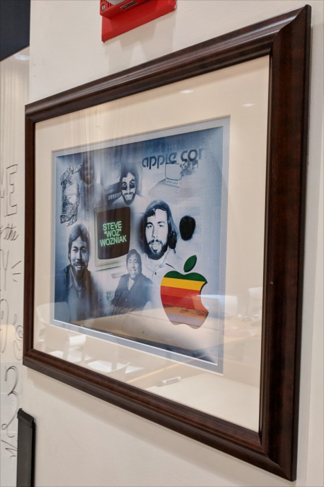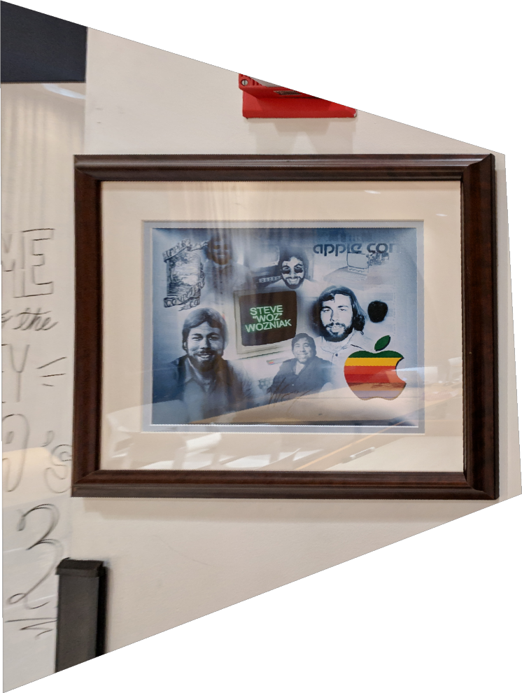woz	rectify woz
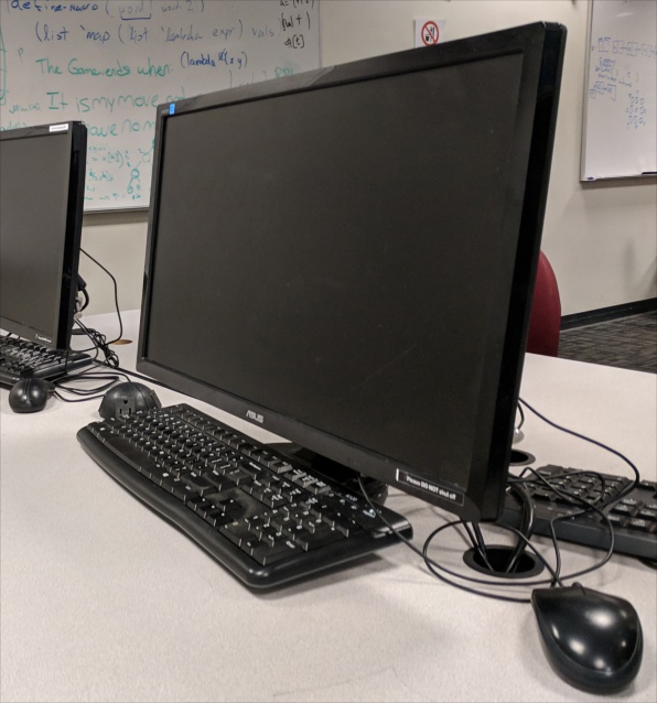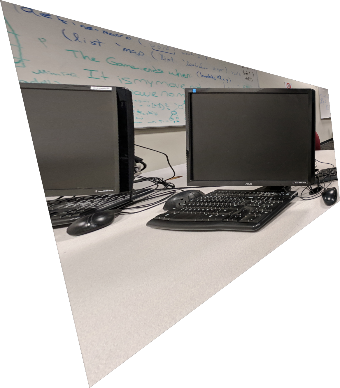desktop	flatscreen

Creating Mosaics

To create a mosaic from two images, we find the homography matrix from corresponding points of the two images, and then warp one of the images to the perspective of the other.

To perform blending on the two images, we performed alpha blending by multiplying the transformed images with a gaussian blurred mask and stored the two images on a large empty image with the proper offsets. The mask of each individual image was also combined to create the alpha channel of the resulting image to allow transparency in the empty parts of the final result.

These did not work out perfectly with minor ghosting and slight mismatches. This is probably due to imprecision selecting correspondences by ginput and shakiness when I was taking the images. Low light photography also contributed to the blurriness.

To conclude, the most important thing we learned in the first part of this project is how homography projections work and can be calculated. It made for an interesting, but slightly tedious project.

Note: I pray that I will never have to use ginput to select a bunch of point correspondences again.

Part 2

In the second part of the project, we performed automatic feature matching to autostitch images without manually selecting corresponding points.

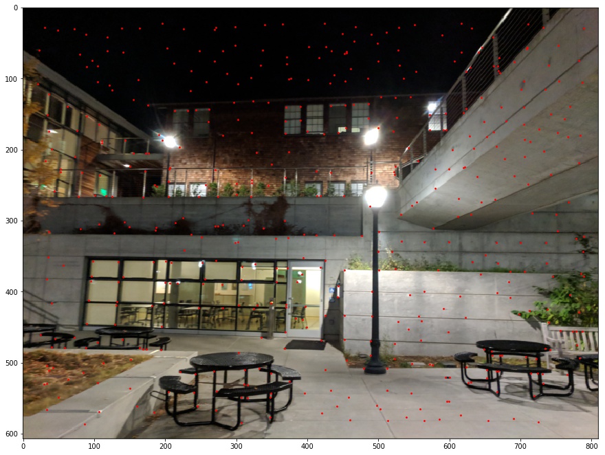
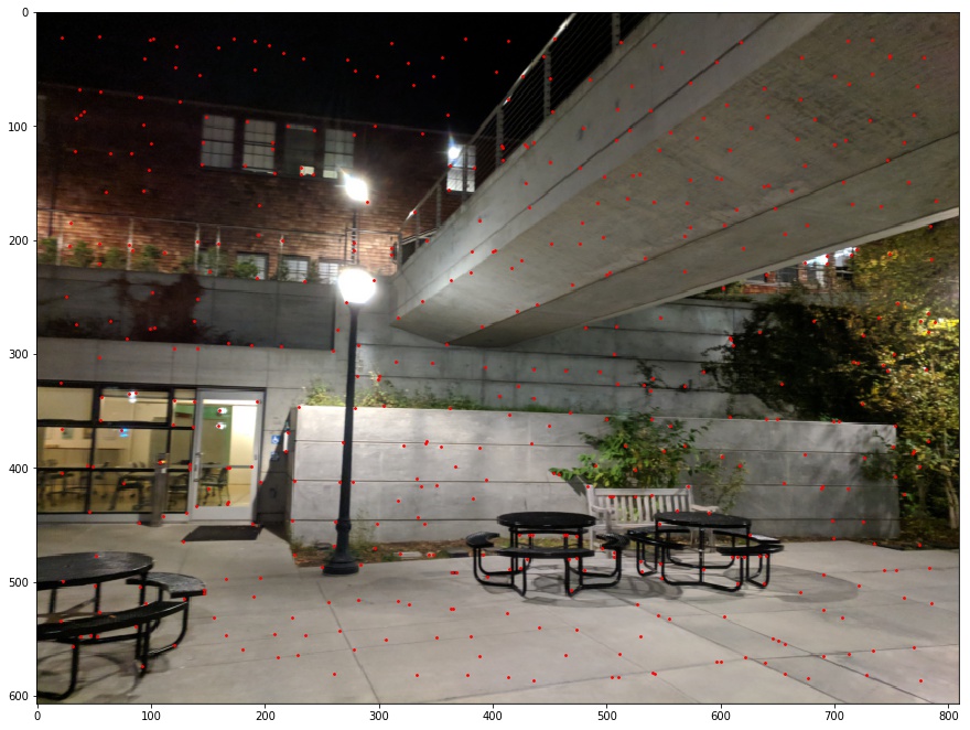
Feature Detector

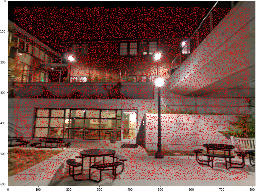
We first needed to find potential interesting features in the two images. We used the Harris Corner Detector algorithm provided by the starter code. The minimum distance between points found needed to be adjusted depending on how large the image is to not innundate the image with too many points as it made later steps very slow. We performed Harris Corner Detection on the greyscale versions of both images.

Non-Maximal Suppression

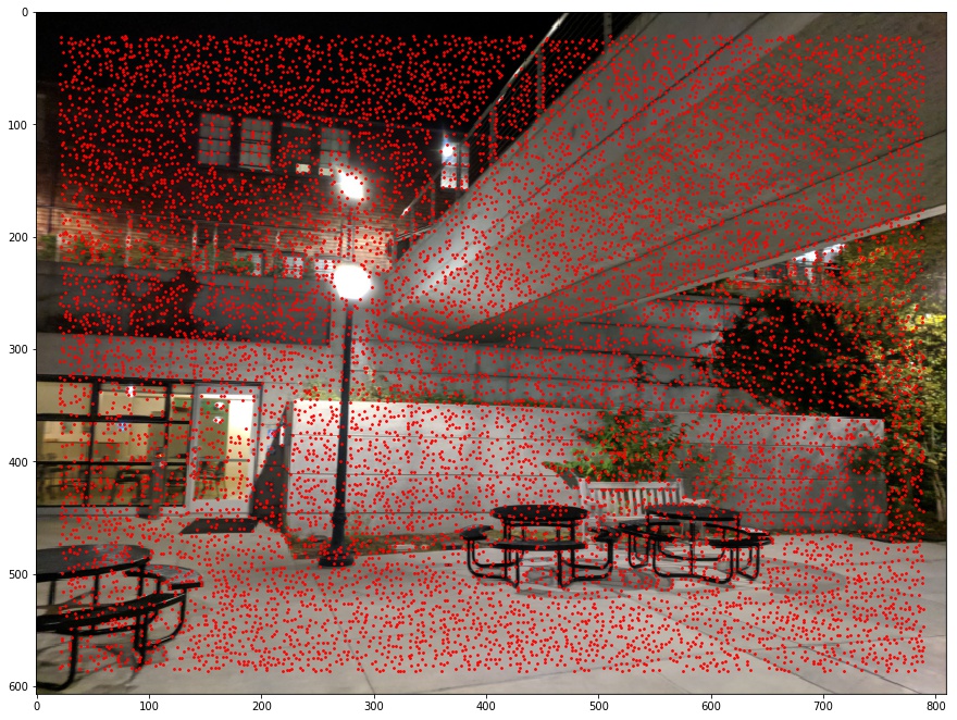
As shown, the corner detector generates too many features to handle. We would like only keep the most revelant ones, while maintaining a relatively even distribution of points across the images. This allows for better matching so the corners with the highest strengths do not clump in very small areas. We follow the constraint below to rank which points to keep based on its radius value $r_i$. $x_i$ represents the current point, $x_j$ represents a point in all the points, $f(x)$ represents the strength of the corner feature, $c_{robust}$ represents a scaling constant.

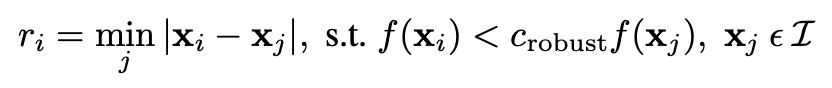
To summarize, we calculate the minimum distance to a point with about as much strength as the current feature. If there are no other points with about as much strength, the distance is infinity. We then choose the points with the highest distance values and suppress the rest. In this project, we suppressed to the top 500 points with the highest radius. In addition, we chose $c_{robust} = 0.9$.

Feature Descriptor

In this step, we extracted features based on feature points in the image. A feature is a 40 by 40 pixel patch in the image centered at each feature point. Again, we extracted features from the greyscale versions of each image. After extracting the features, we resized the patches to be 8 by 8 for more concise feature descriptions. Finally, we subtracted the features by the mean patch pixel value and divided by the standard deviation of the pixel value to account for bias and gain. As a final post-processing step, we reshaped each 8 by 8 feature into a dim 64 vector to work with.

Feature Matching

With descriptions for each feature, we could now match potential corresponding features in the two images to stitch. To find similar features, we first started with nearest neighbor, getting the squared distance between all the feature descriptions. For thresholding which matches to let through, we use Lowe's approach of thresholding on the ratio of each feature's first nearest neighbor to its second nearest neighbor. For the most part we used a thresholding value of 0.6. If the ratio of nearest neighbors for a feature point was under the threshold, we treated its first nearest neighbor to be a good potential match.

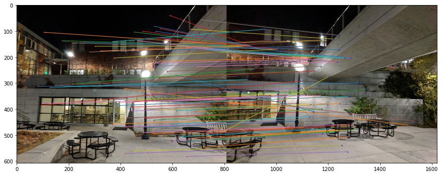94 matching features found

RANSAC

Although we now had corresponding points, not all the matches were necessarily correct. Since there are many outliers, we try our best to find a homography matrix that works for the most matches. This process is is called Random Sampling Concensus (RANSAC). We choose a random sampling of 4 correspondences to calculate a homography matrix, and find the SSD of the warped points from the first image through the homography matrix and those of the second image. We consider a point matching to be an inlier if the SSD error is below a certain thresholding value epsilon. Throughout the project, we used an epsilon value of 1.5 and 100 iterations. We then repeat the process a set number of iterations and keep track of, from all the iterations, the largest set of inliers from a randomly sampled homography matrix. We then calculate the final homography matrix from this largest set of inliers.

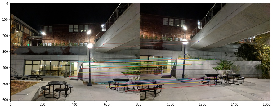Remaining 31/94 matches used after RANSAC

With the homography matrix found, we could now perform the process from part 1 to stitch mosaics.

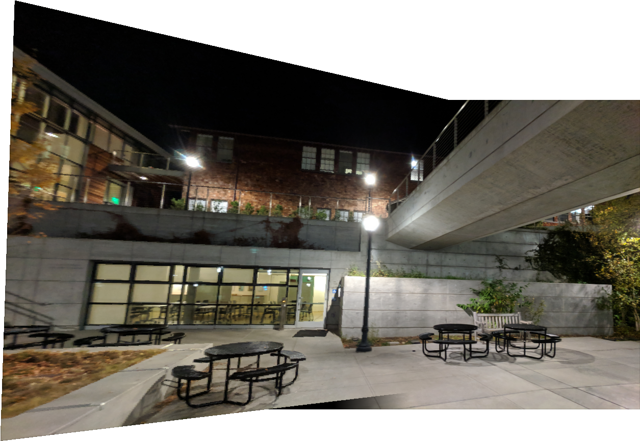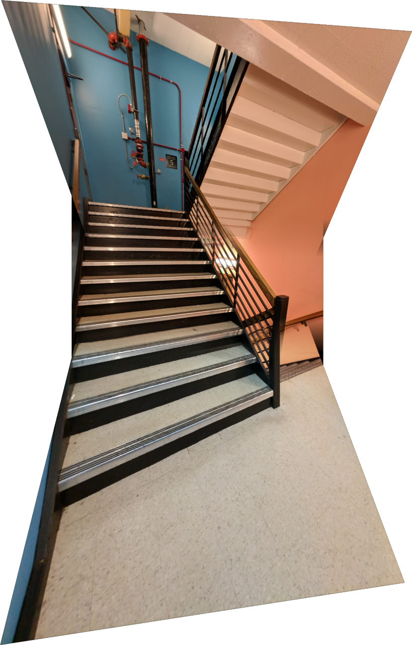
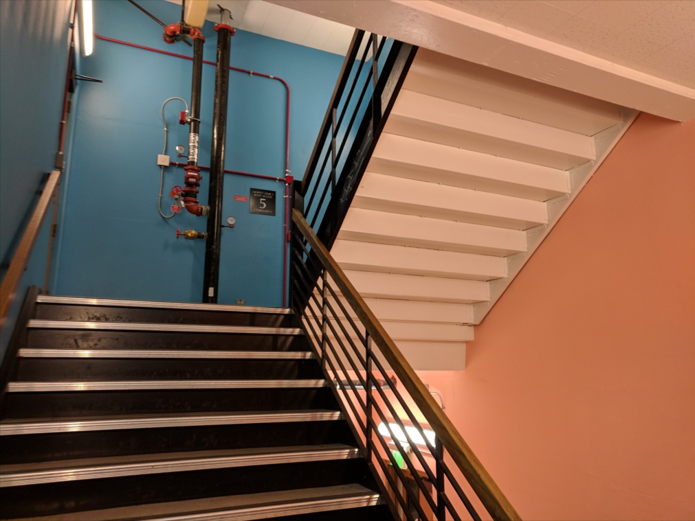
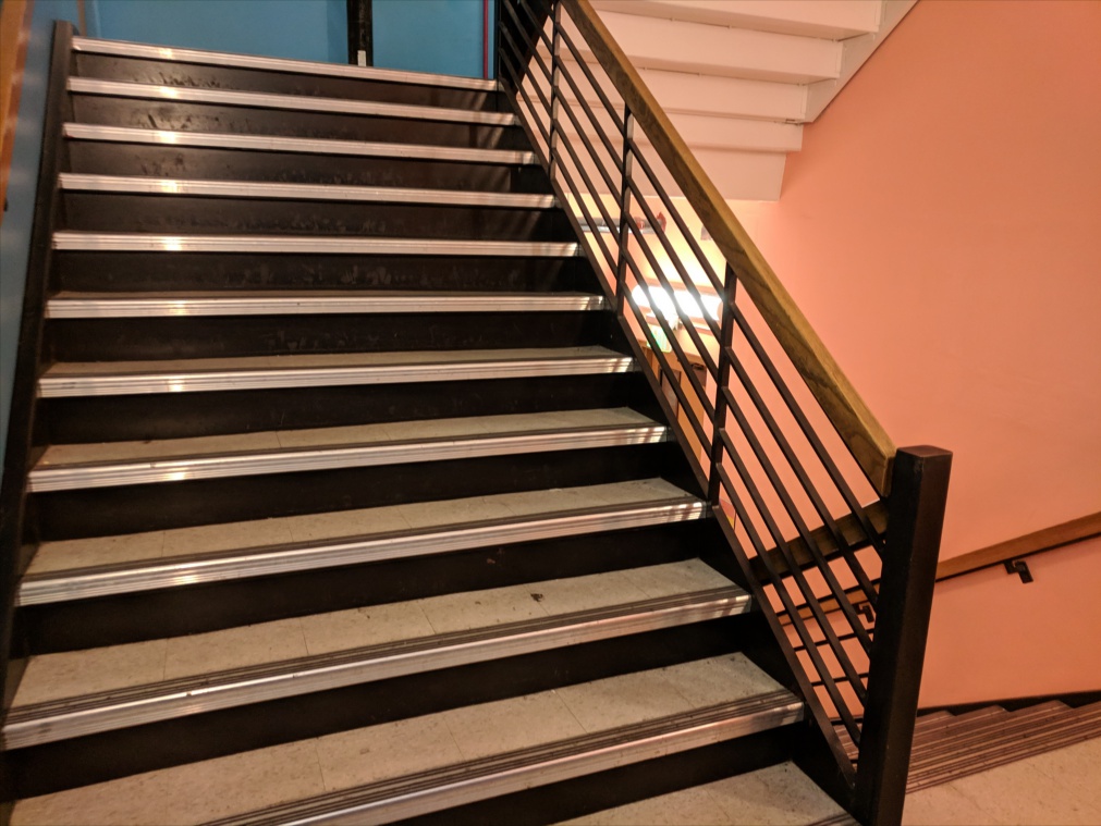
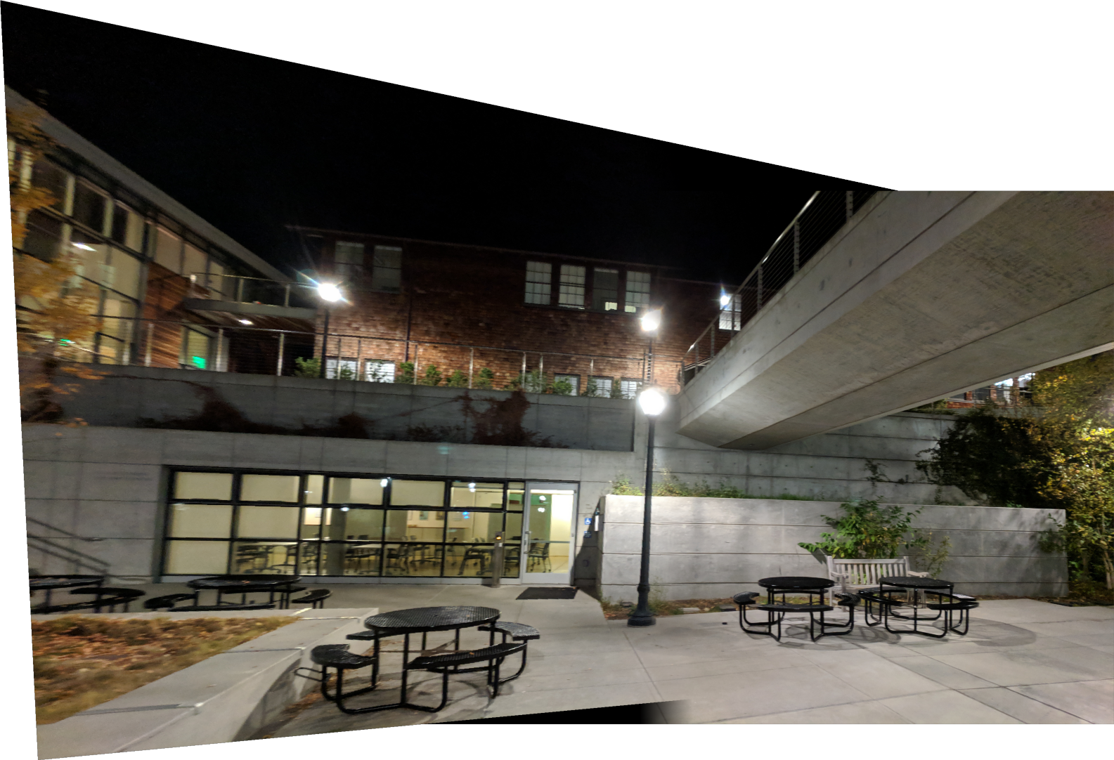
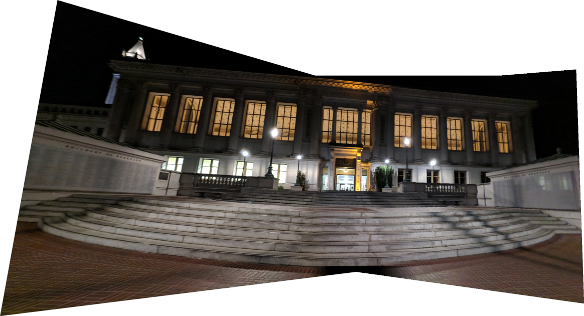
Manual point selection	Auto-stitched selection

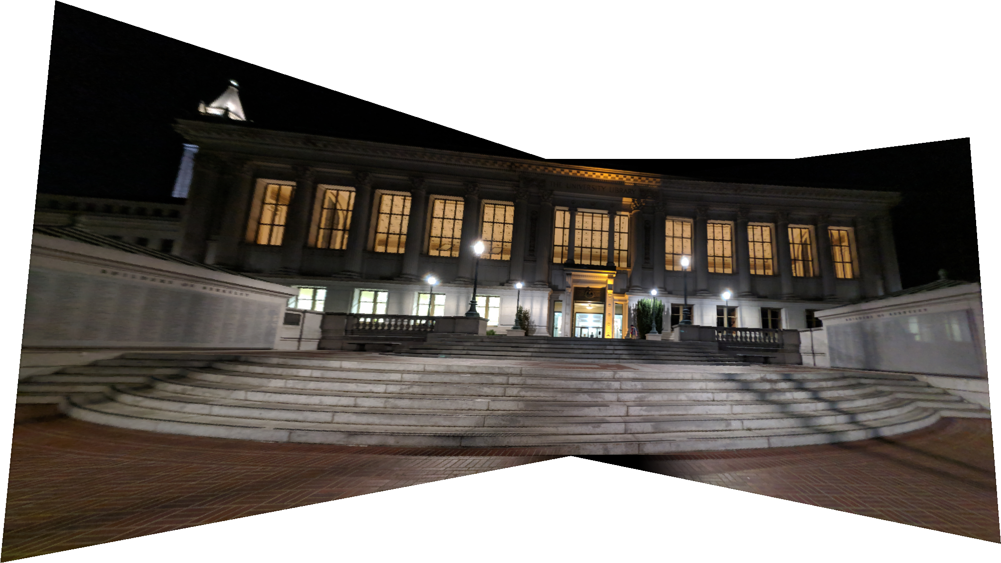Manual point selection	Auto-stitched selection

Manual point selection	Auto-stitched selection

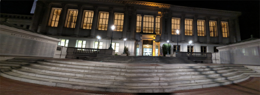
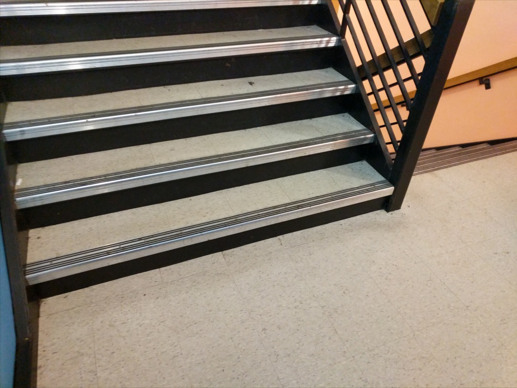
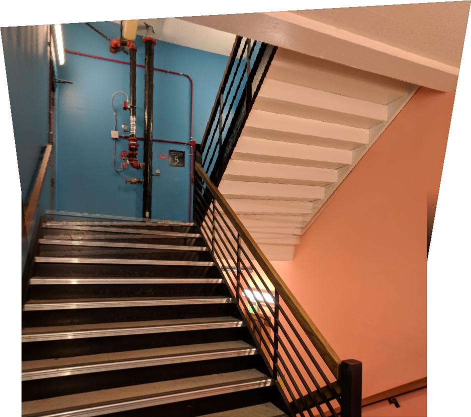
The staircase image from part 1 proved exceptionally difficult, with auto-stitching having a hard time finding correct matches with the default settings used. We hypothesized that this was due to feature patches being too small as the image has a lot of different features that look similar to each other (corners on staircase steps that might look the same through a 40 by 40 patch). To remedy this, we increased the patch size to 80 by 80 to produce a workable but questionable quality merge. For the other images, the results seem relatively similar to that of the manually feature selected images. Other probably causes of error include the relatively low quality low light phone images affecting the auto-stitching algorithm in retrieving features. In addition stitching images with higher resolution most likely require increasing patch size and corner detection minimum distance maintain relative patch descriptor robustness while not slowing the algorithm down with too many points to suppress. It would have been nice to have a nicer camera with a tripod to get better images. However overall, the auto point selection and mosaic stitching worked pretty well.

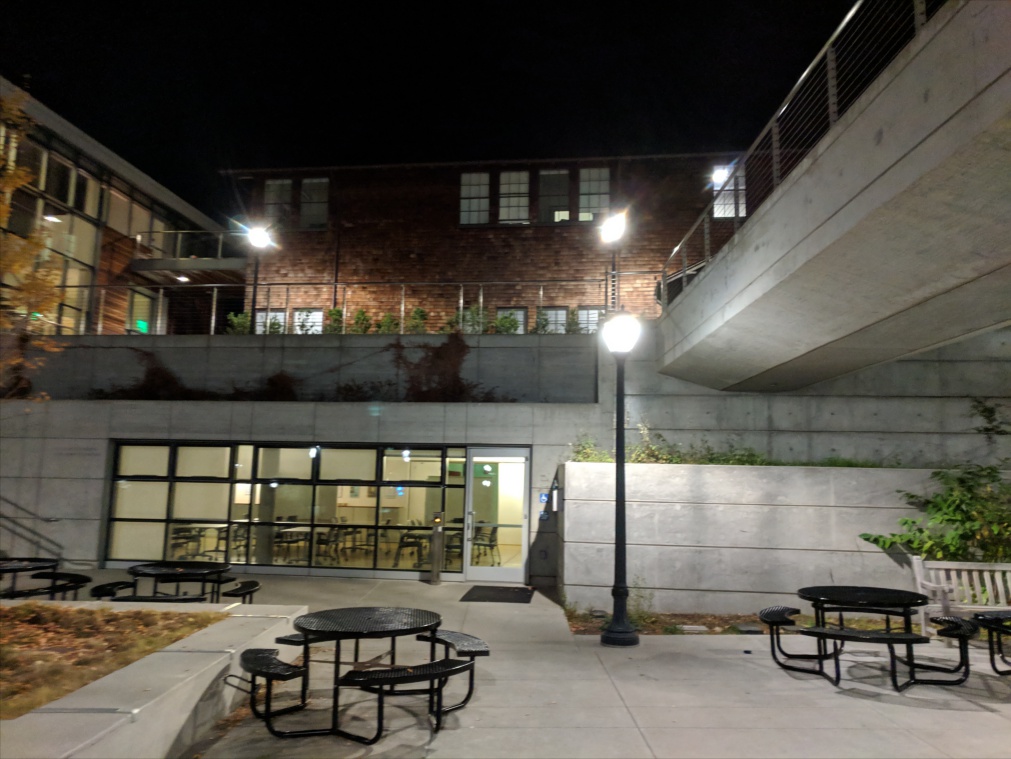
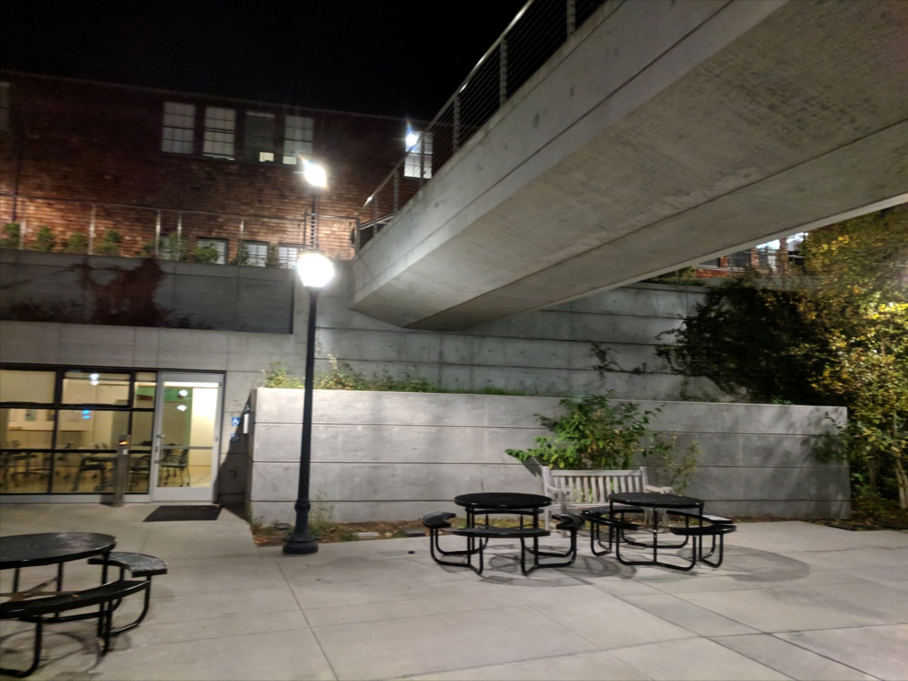
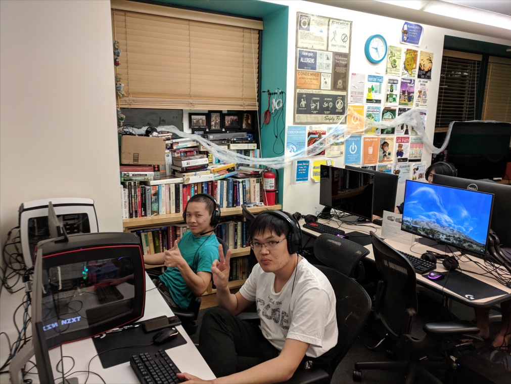
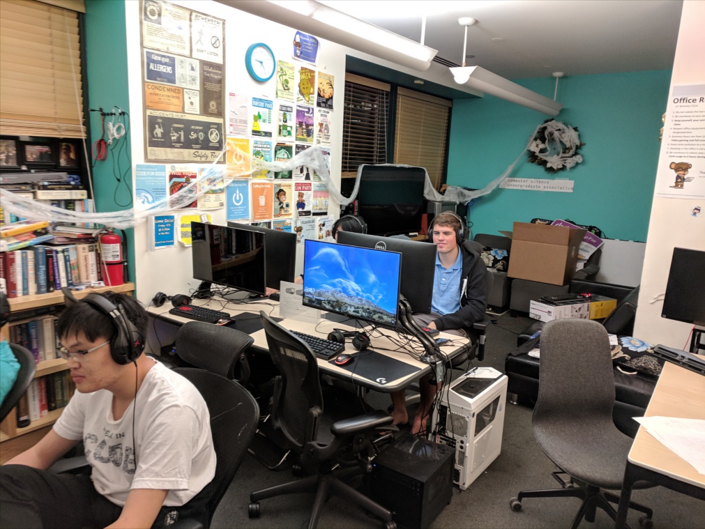
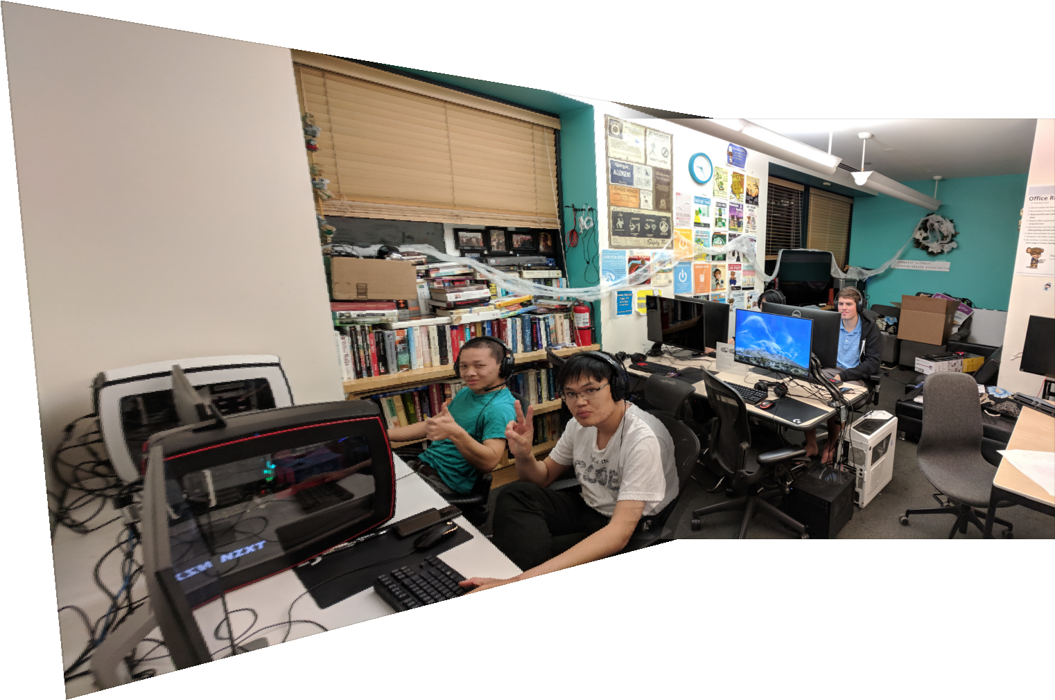
Extra auto-mosaics

Night at the CSUA.

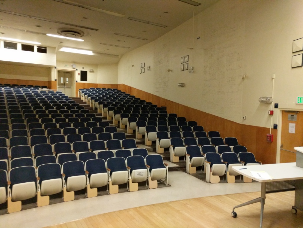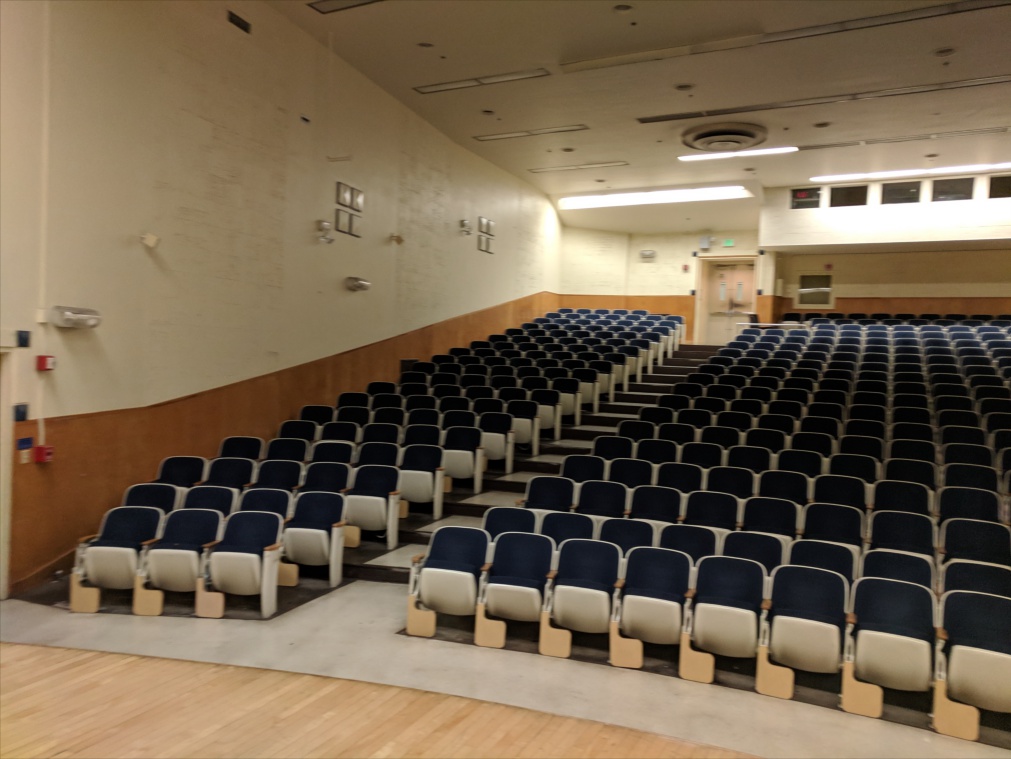
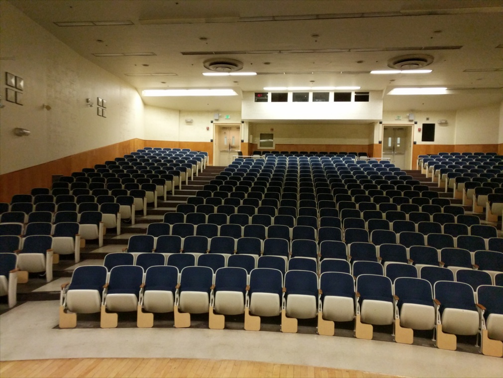
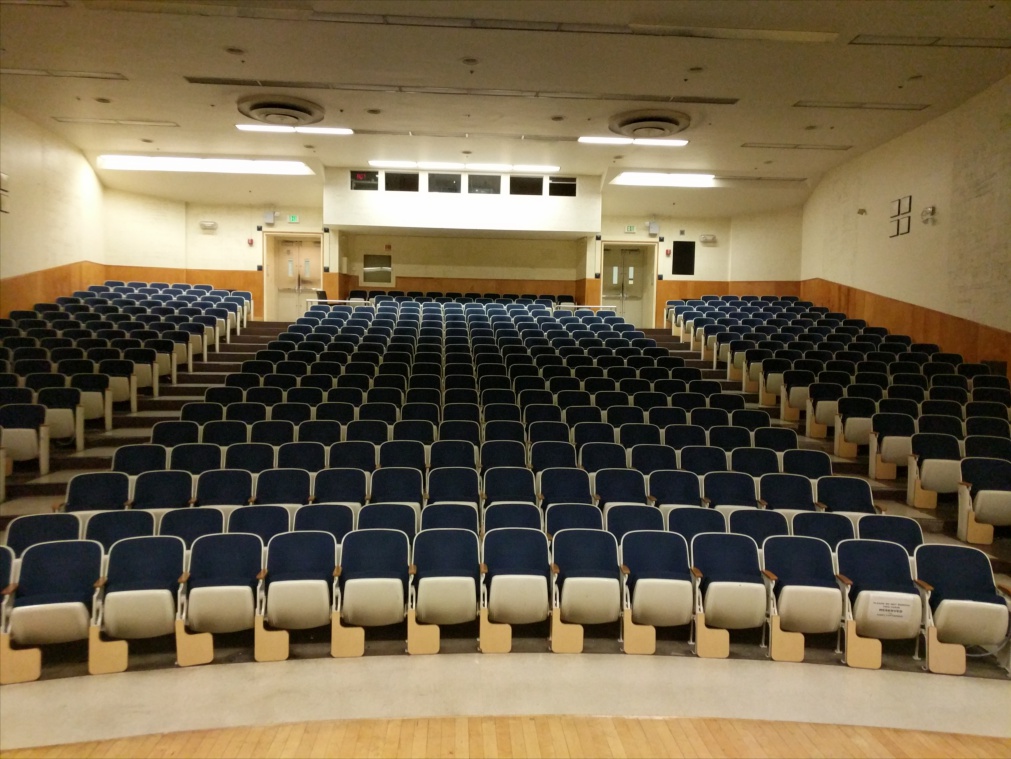
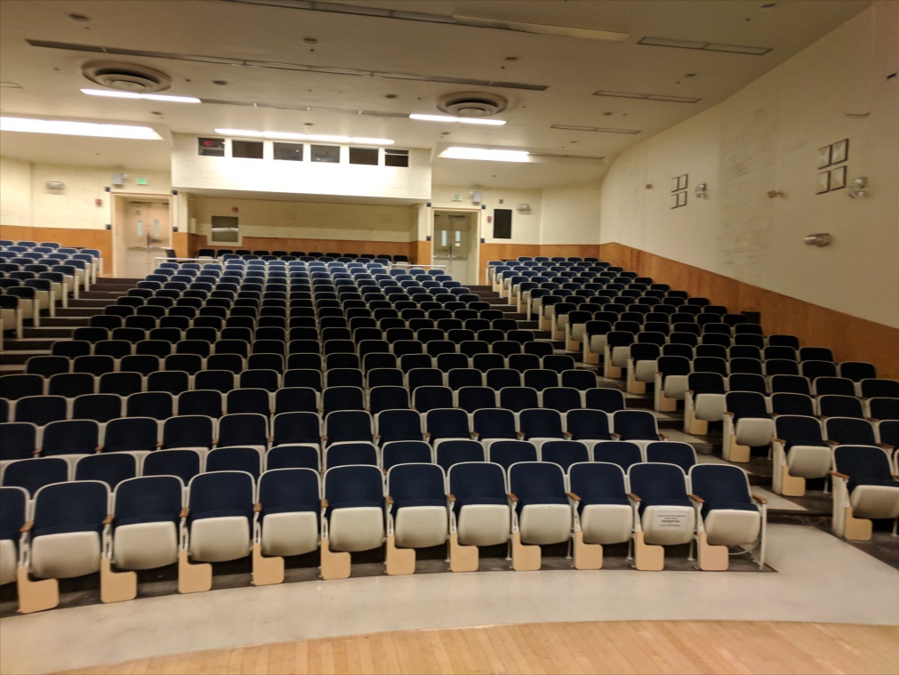
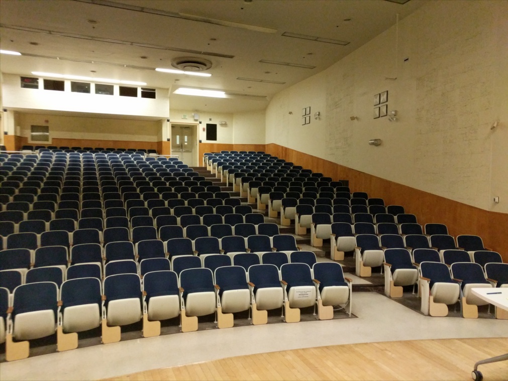
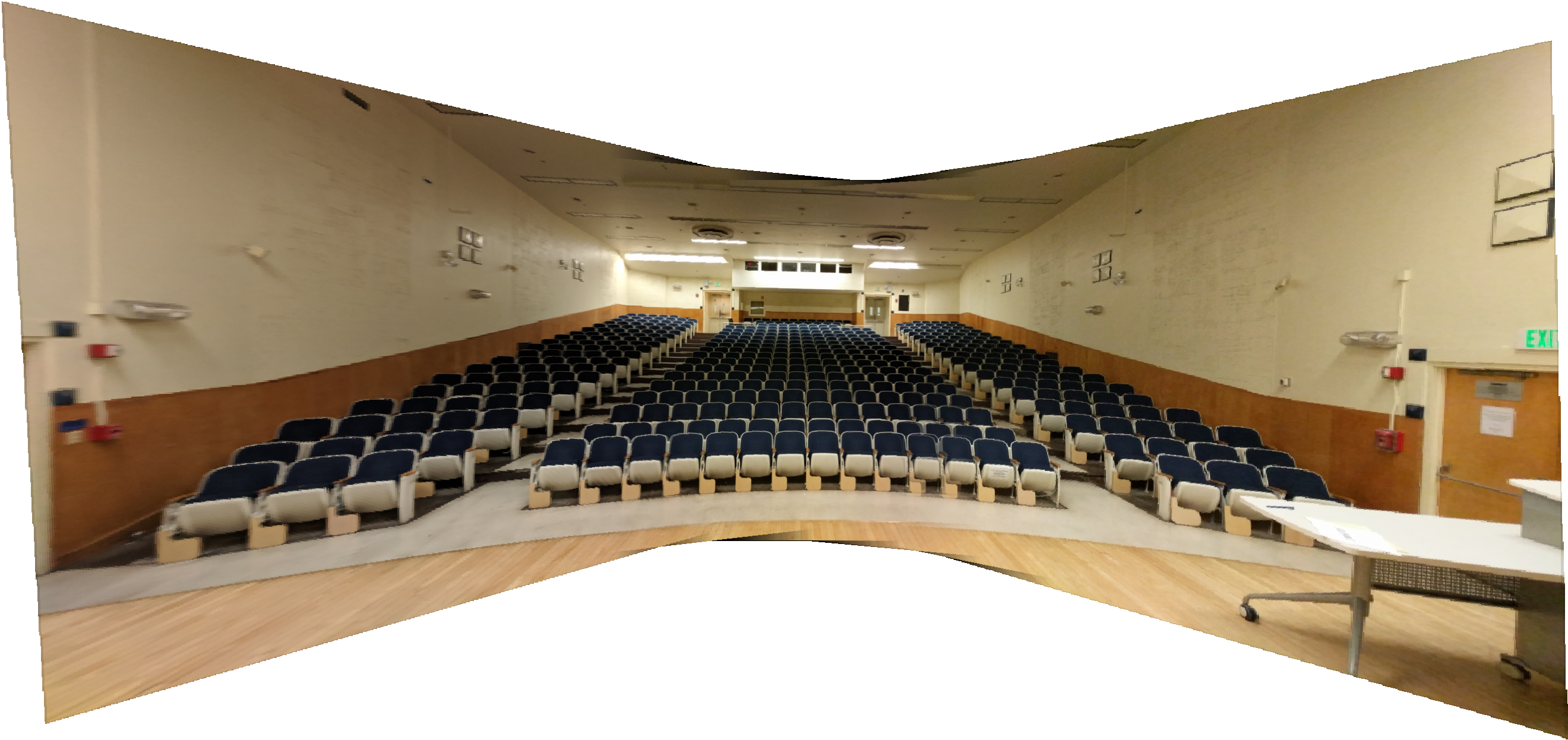Home to the worst chairs.

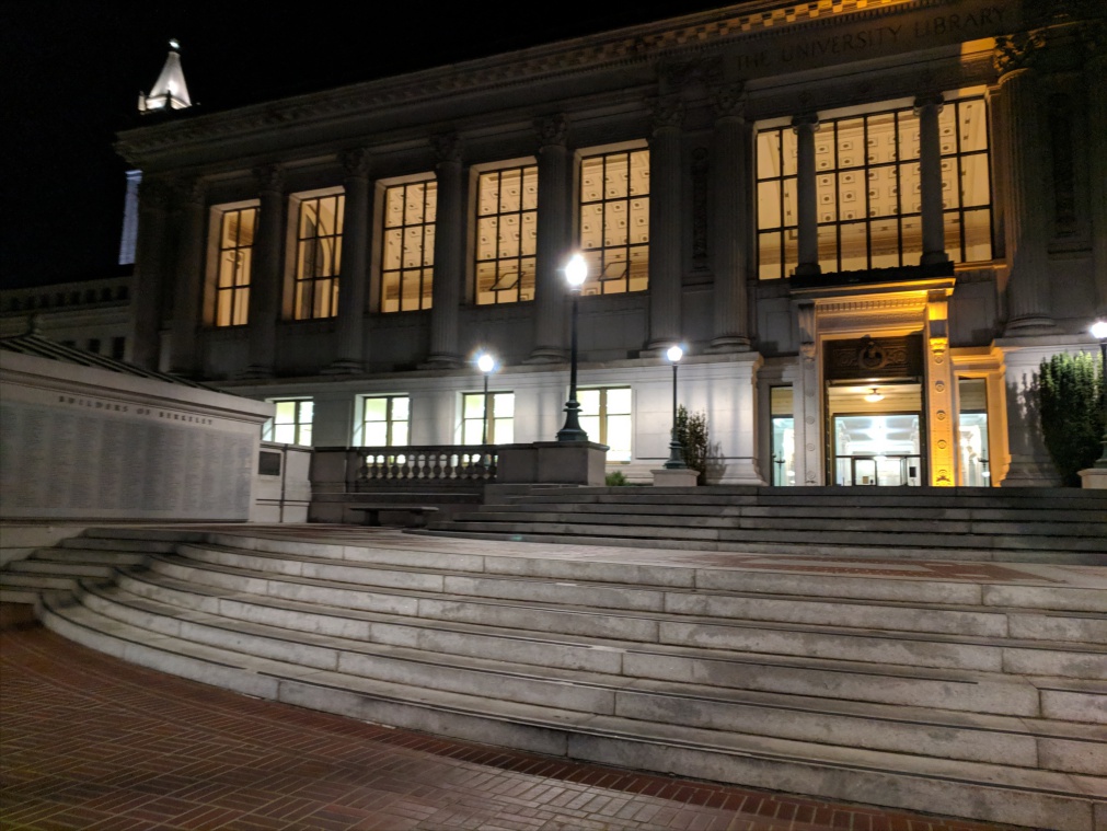
The whole auto feature detection pipeline was the coolest thing I learned from this project. It definitely made stitching Dwinelle actually feasible and much better than my clicking.