1. I first computed the Homography matrix H that mapped the correspondences between the two images to warp the coordinates of Image 1 to the alignment of Image 2.
2. I applied H to the four corners of Image 1, and got a rectangular bounding box of the warped corners.
3. Within each coordinate of the rectangular bounding box, I applied H^-1 to get the corresponding coordinates from Image 1 to get the pixel from.
4. I used interpolation if the recovered coordinates were decimals and not integers. If the recovered coordinate was not found within Image 1, I would set the pixel value to 0 (this was observed for the cases when I was doing an inverse warp on a coordinate within my bounding box that was not contained within the polygon enclosed by the warped corners)
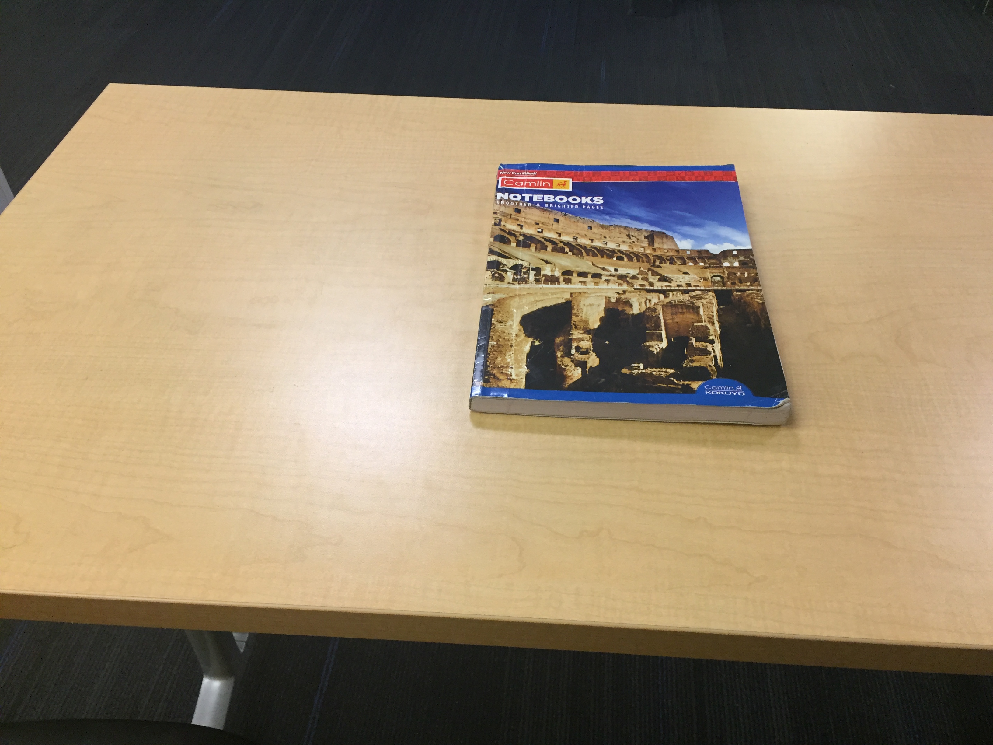
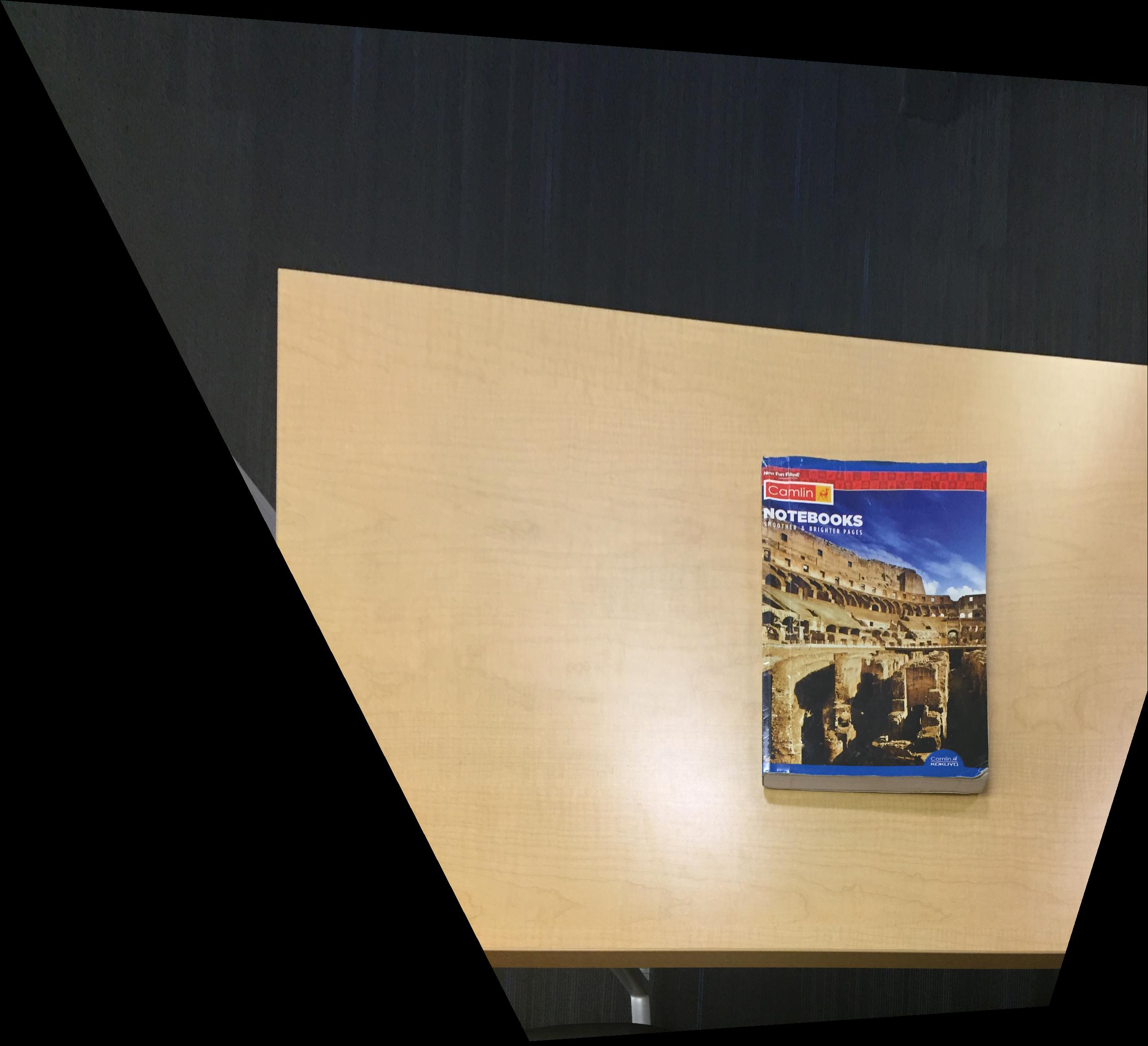
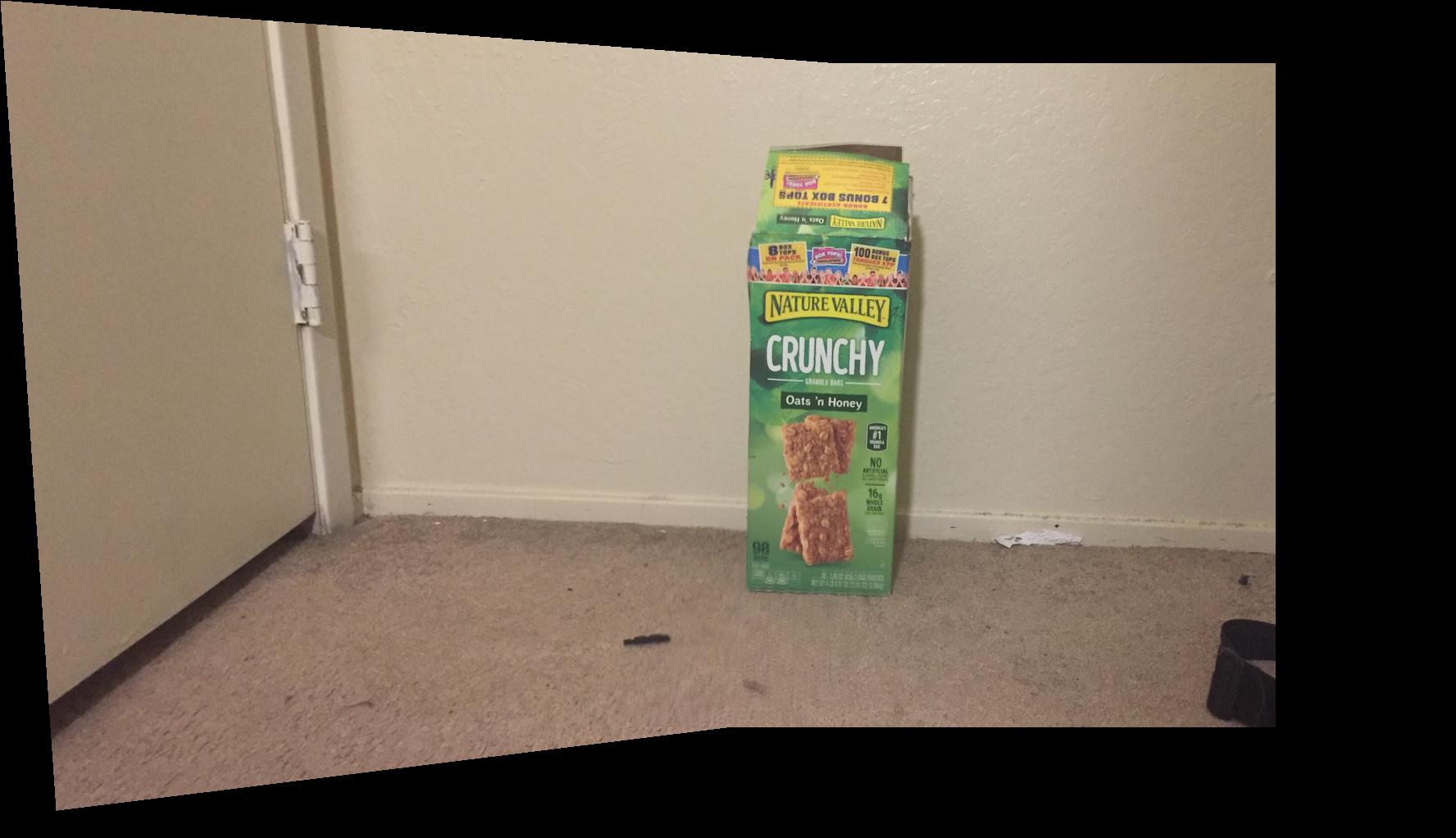
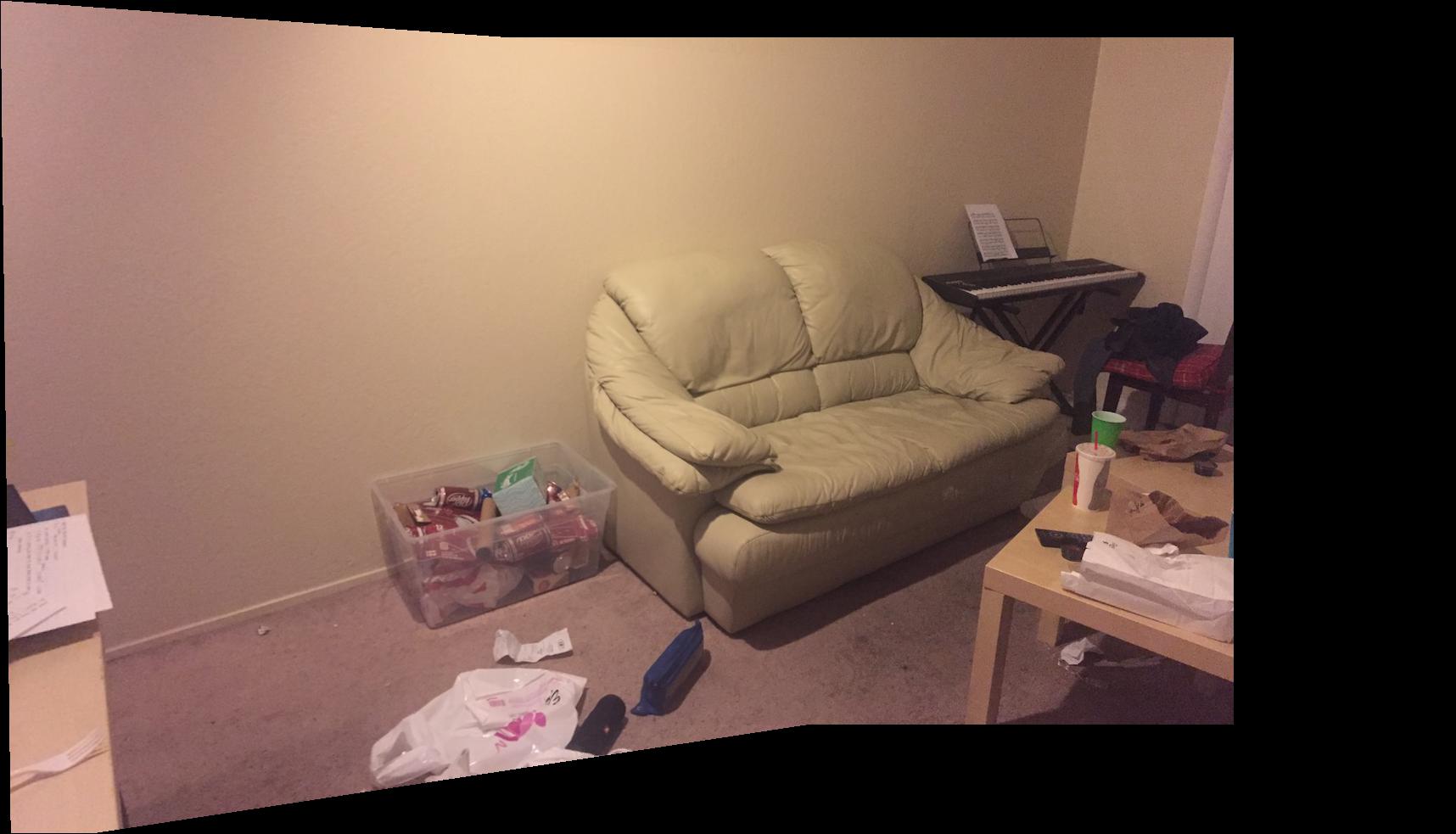
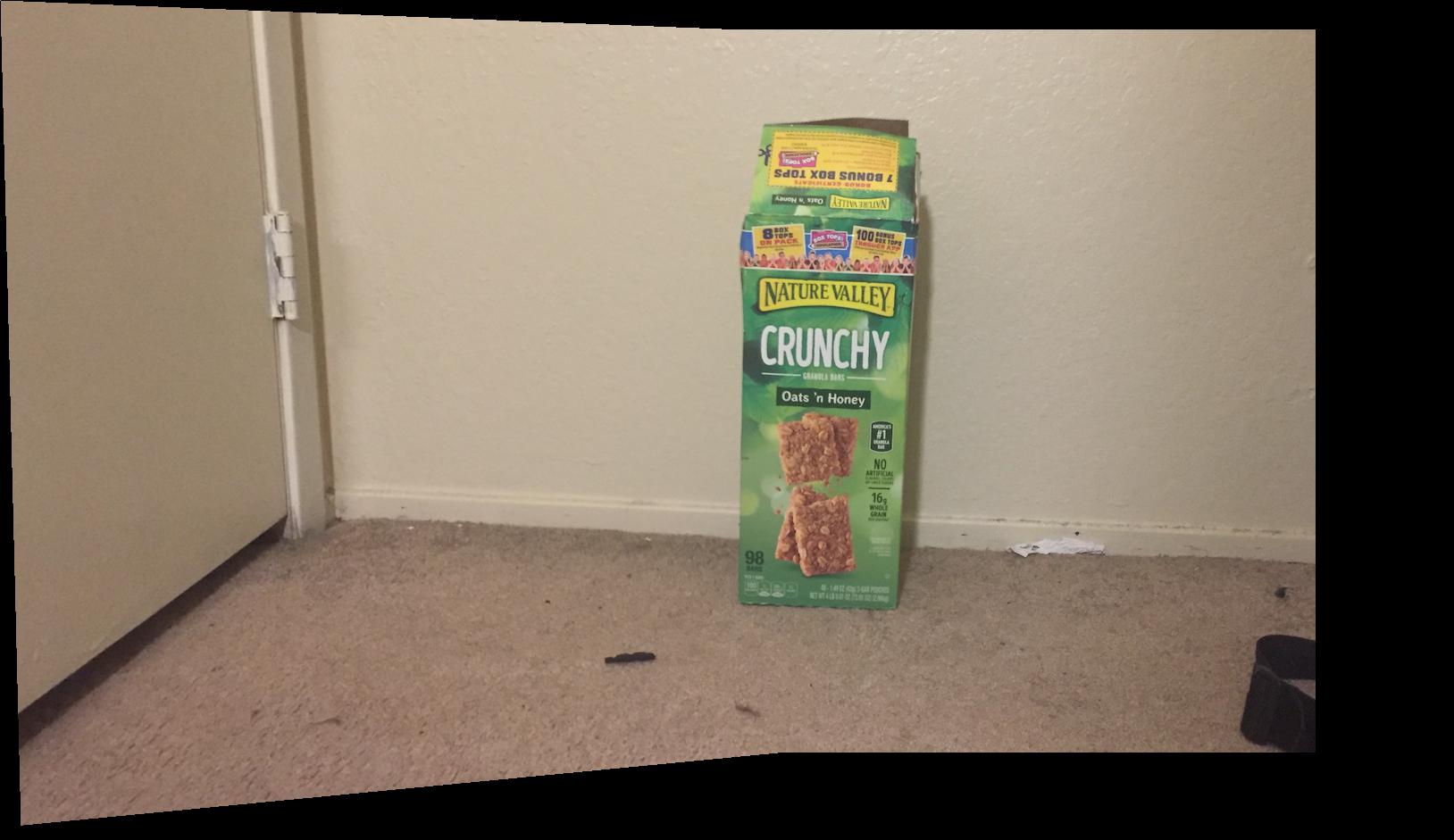
Rectified images can be seen below:
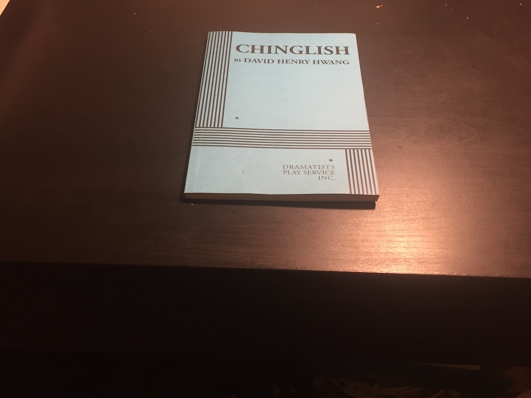
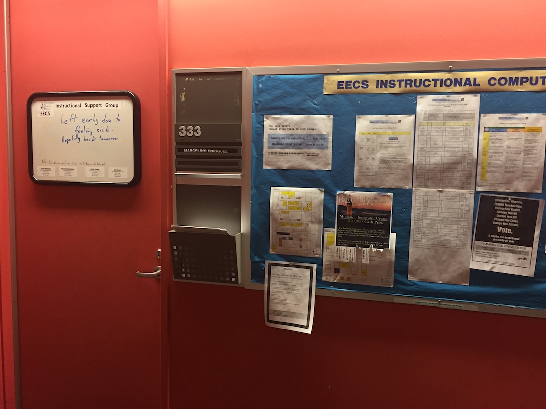
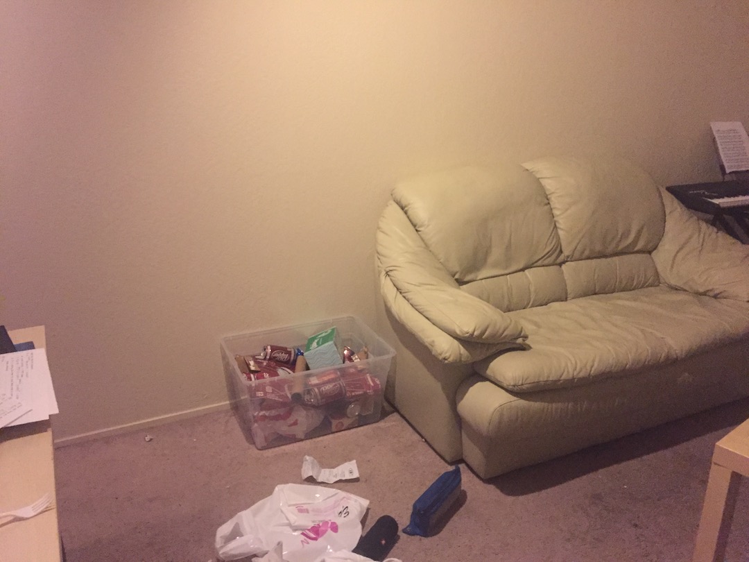
Another pair of original and rectified images is as follows:

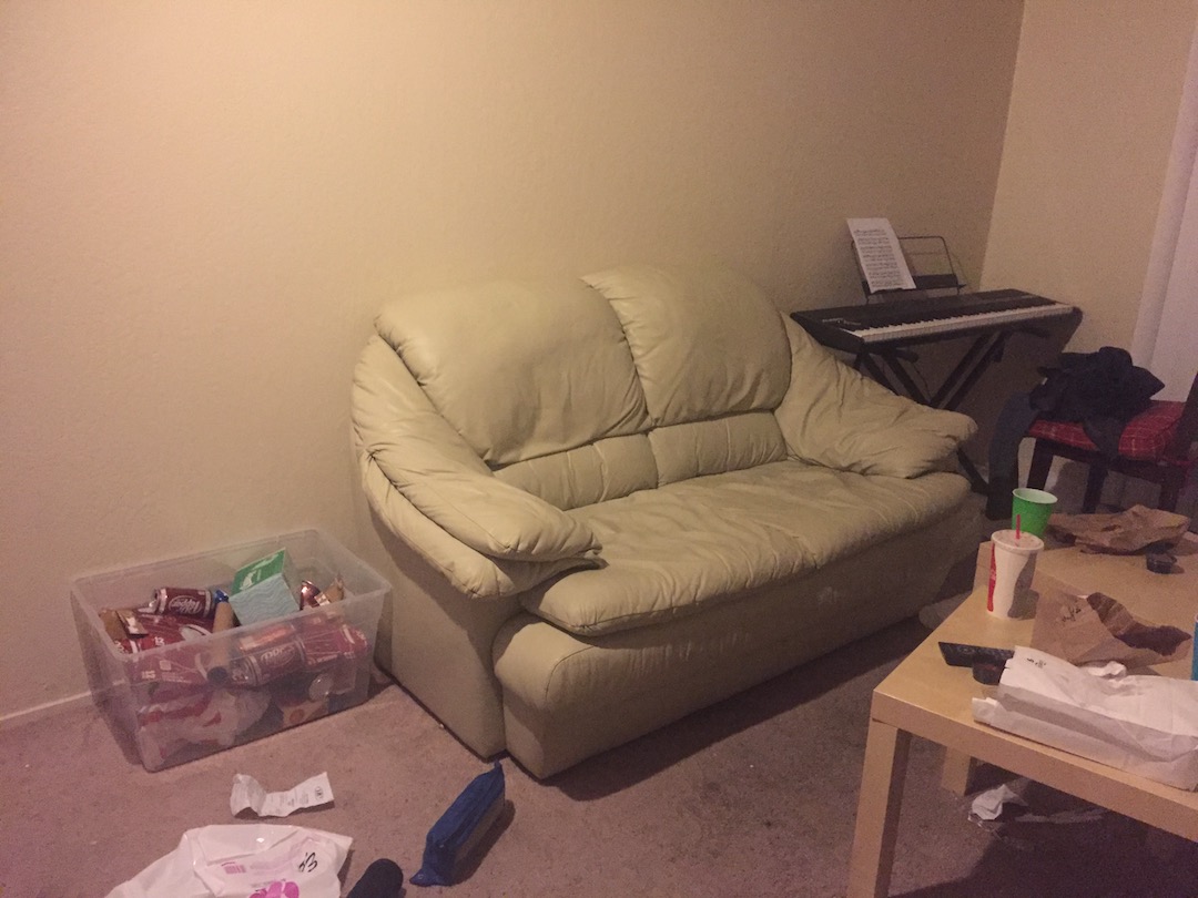
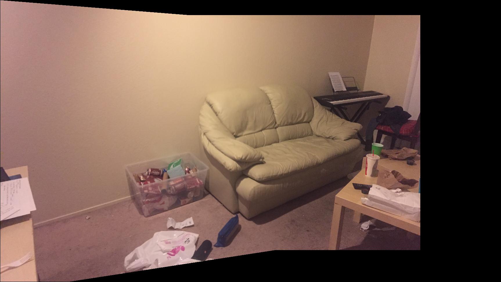
The first mosaic is as follows:
The second mosaic is as follows:
The third mosaic is as follows:
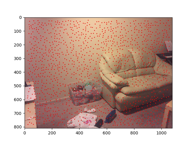
The Harris Corner Detector returns a lot of corners, and using all of the corners would slow computations down significantly. Ideally, we would want to select a subset of these corners, and we would want this subset of corners to be evenly distributed across the image.
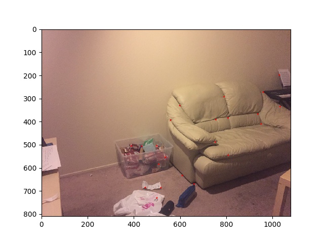
In order to obtain a subset of corners that are evenly distributed across the image, I implemented the Adaptive Non-Maximal Suppression Algorithm. For each Harris corner A, I defined the suppression radius as the closest distance from Harris corner A to another Harris corner B such that the corner strength of A is less than 0.9 times the corner strength of B. I then picked the 400 Harris Corners with the largest suppression radius.

The corners chosen in the example image above do seem evenly spaced
To extract feature descriptors, I first took a 40 by 40 Gaussian blurred window around each corner from the image. For eeach patch, I subsampled every 5th pixel to get a 8 by 8 patch. Each patch was then bias/gain normalized so that it was zero mean and had unit standard deviation. I then computed a matrix of pairwise SSD distances between each pair of these bias/gain normalized patches, in order to eventually match feature spaces together. For each patch, I looked at the distance to the nearest neighbor (let's call this distance 1-NN), and the distance to the second nearest neighbor (let's call this distance 2-NN). I computed the ration 1-NN/2-NN, and determined a correspondence between a patch and its nearest neighbor only if 1-NN/2-NN for that patch was less than 0.6. If a correspondence was determined between a patch and its nearest neighboring patch, I said there was a correspondence between the Harris corners those patches corresponded to.


If we look closely at the corners displayed on each of the images above, we can see that they do correspond to the same points of interest.
In order to estimate the Homography needed to warp one image to another, I implemented the RANSAC algorithm. Without Loss of Generality, let's assume our two images are called Image 1 and Image 2, and we trying to warp Image 1 to the alignment of Image 2. In this algorithm, for each iteration of a pre-specified number of iterations (10000 iterations in this case), we randomly sample 4 correspondences out of those identified from the earlier section. We then compute a exact homography H between these 4 correspondences, and then, we apply this Homography to all the corners from Image 1 in the correspondences determined earlier. If applying H to a point from Image 1 gives us a point that matches closely with the corresponding point from Image 2, the point obtained is considered to be an inlier - this was determined by computing the Euclidean Distance between the coordinates of warped point from Image 1 and the expected point in Image 2, and considering it to be an inlier if the Euclidean Distance was less than 1, i.e., if the warped point was less than 1 pixel away from the expected point in Image 2. I counted the number of inliers for every iteration, and kept track of the largest set of inliers, and the correspondences that gave us those inliers. I then computed the Homography to warp Image 1 to the alignment of Image 2 using the correspondences that gave us the largest set of inliers, and determined this to be the Homography needed to warp Image 1 to the alignment of Image 2.
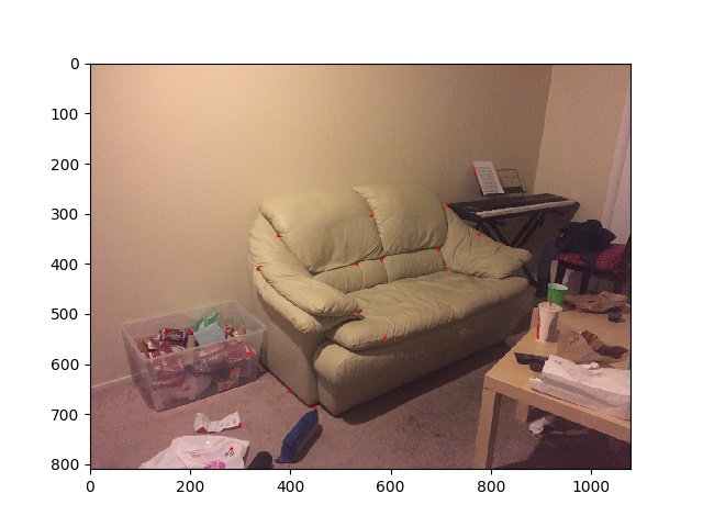
Only a subset of the matched corners has been chosen by RANSAC
Without Loss of Generality, let's assume our two images are called Image 1 and Image 2, we trying to warp Image 1 to the alignment of Image 2. Using the Homography computed from RANSAC, I warped Image 1, using inverse warping as in Part A. I then blended the warped Image 1 with Image 2 as in Part A, to get a Mosaic.
The first mosaic is as follows:
The automatically stitched mosaic is more visually appealing, as the manually picked correspondences may have been slightly misaligned, whereas this would not be the case with the automatically defined correspondences.
The second mosaic is as follows:
The automatically stitched mosaic is more visually appealing, as the manually picked correspondences may have been slightly misaligned, whereas this would not be the case with the automatically defined correspondences.
The third mosaic is as follows:
The automatically stitched mosaic is more visually appealing, as the manually picked correspondences may have been slightly misaligned, whereas this would not be the case with the automatically defined correspondences.