Overview
This assignment used image warping with a “cool” application of image mosaicing. I took photographs to create an image mosaic by registering, projective warping, resampling, and compositing them. Along the way, I learned how to compute homographies, and how to use them to warp images.
Part 1: Shoot the Pictures
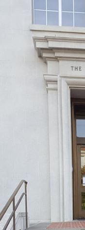
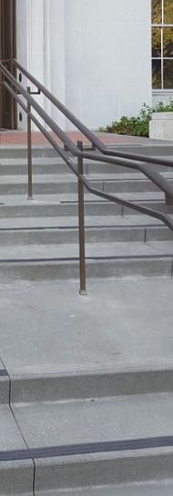
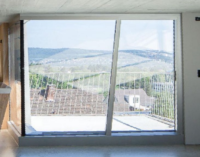
I shot multiple photographs so that the transforms between them are projective (a.k.a. perspective). To do this, I shot images from the same point of view but with different view directions, and with overlapping fields of view. Another method I used was to shoot pictures of a planar surface (e.g. a wall) or a very far away scene (i.e. plane at infinity) from different points of view. I acquired my pictures using a Sumsung Galaxy S6 phone camera with the highest allowable resolution setting. I tried to shoot as close together in time as possible, so your subjects don't move on you, and lighting doesn't change too much. Additionally, I used identical exposures and focus locking so as to maximize the image brightness in the overlap region and overlapped the fields of view significantly to between 40% to 70% as recommended. I took a picture of building exteriors/entranceways and forests.
ORIGINAL IMAGES USED FOR RECTIFICATION AND WARPING
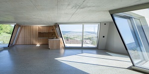
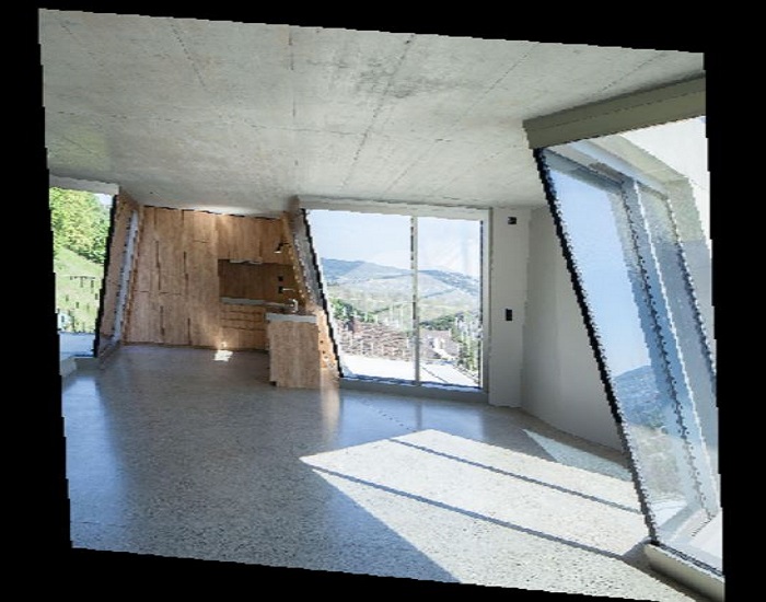
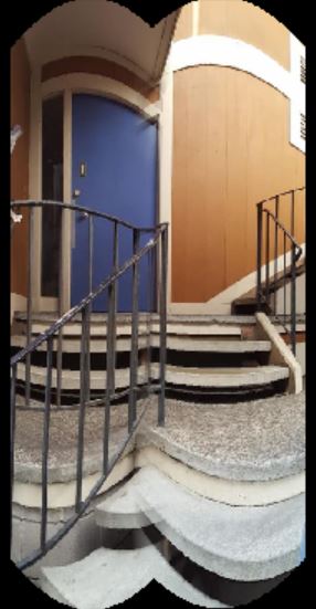
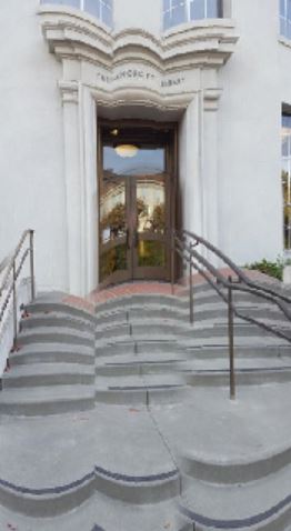
Fancy Building Room
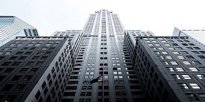
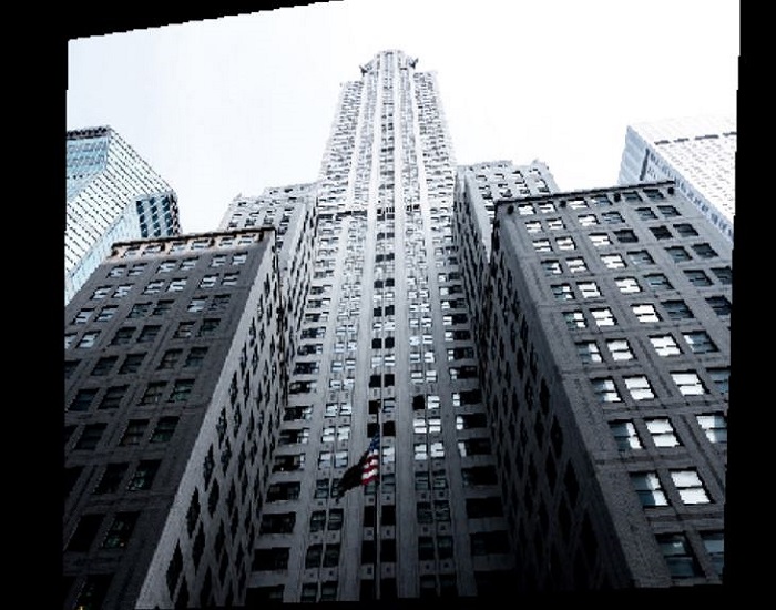
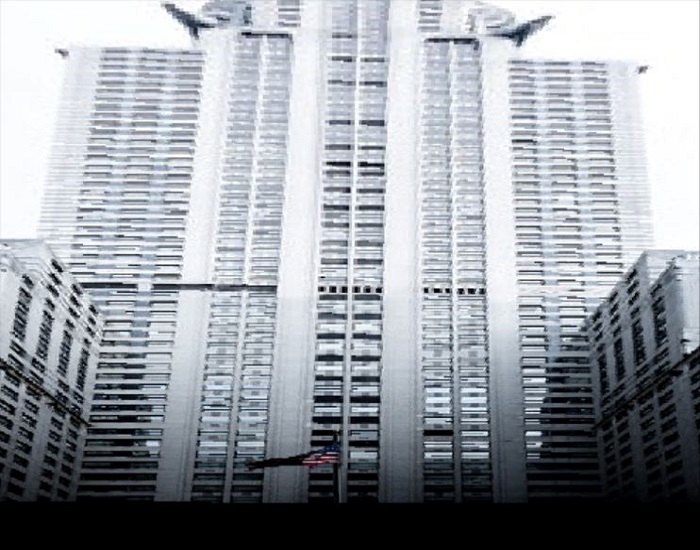
Chyrsler Building, New York
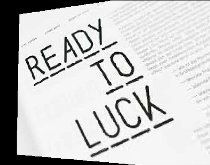
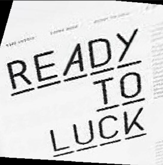
Book
ORIGINAL IMAGES USED FOR PLANAR BLENDING AND CYLINDRICAL BLENDING
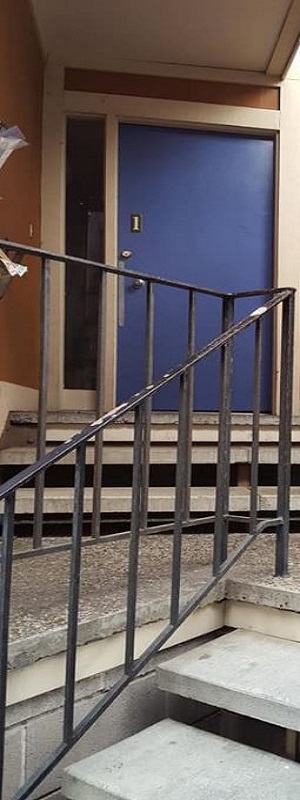
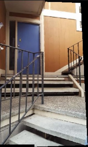
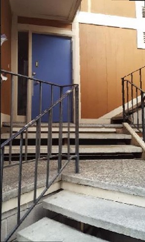
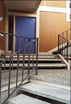
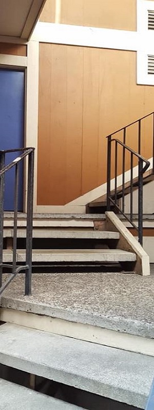
Apartment Building Left View
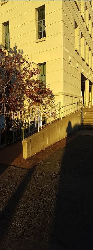
Apartment Building Right View
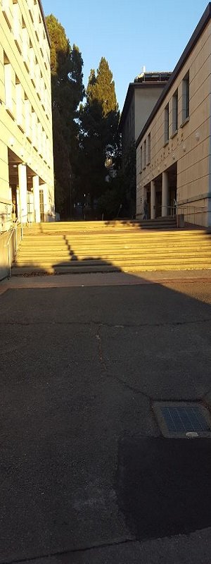
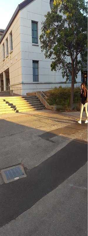
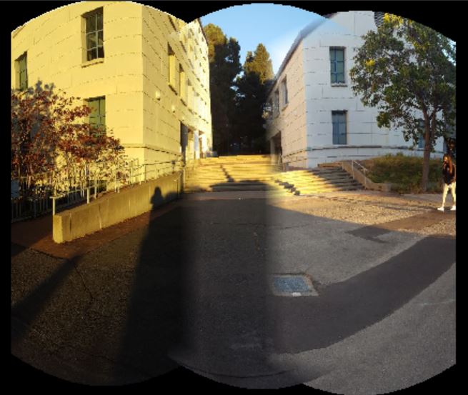
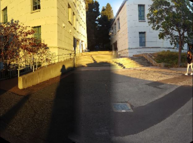
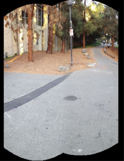
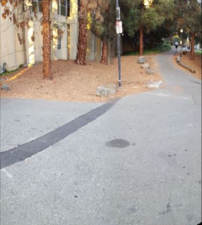
Genetics & Plant Biology Building Left View
Genetics & Plant Biology Building Center View
Genetics & Plant Biology Building Right View
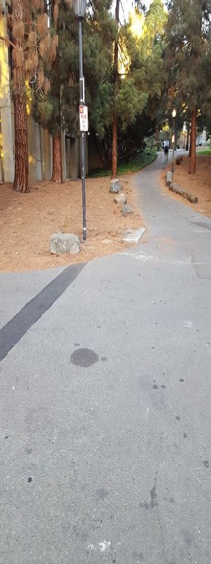
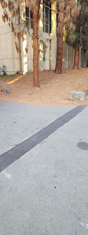
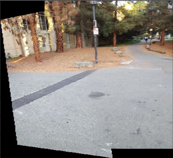
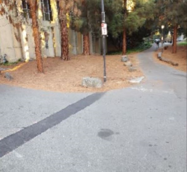
Trees Right View
Trees Left View
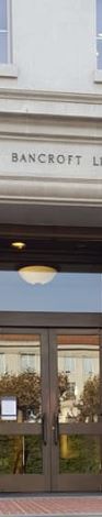
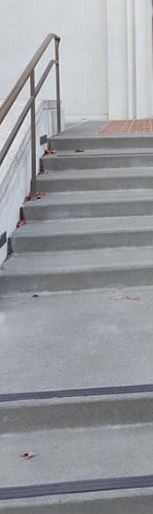
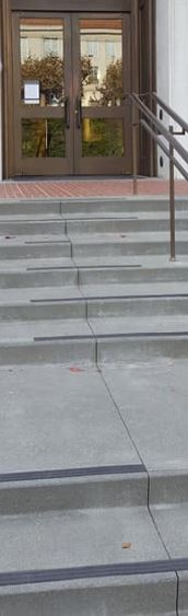
ORIGINAL IMAGES USED FOR FULL 360 DEGREE CYLINDRICAL BLENDING
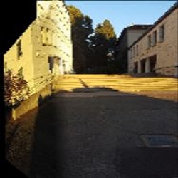
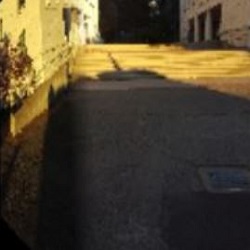
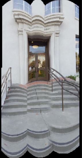
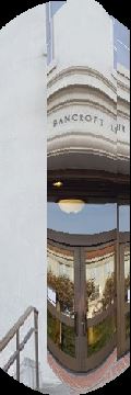
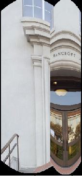
Bancroft Library View 1
Bancroft Library View 2
Bancroft Library View 3
Bancroft Library View 4
Bancroft Library View 5
Bancroft Library View 6
Recover Homographies
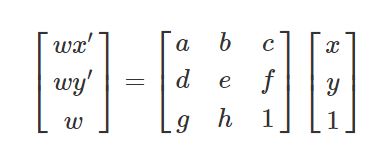
Before warping the images into alignment, I recovered the parameters of the transformation between each pair of images, with the transformation being a homography defined by: p’=H*p, where H is a 3x3 matrix with 8 degrees of freedom (lower right corner is a scaling factor and can be set to 1). This can be described by:
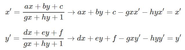
I recovered the homography through a set of (p', p) pairs of corresponding points taken from the two images. Given that
p' is not at infinity, x' and y' can then be expressed as:
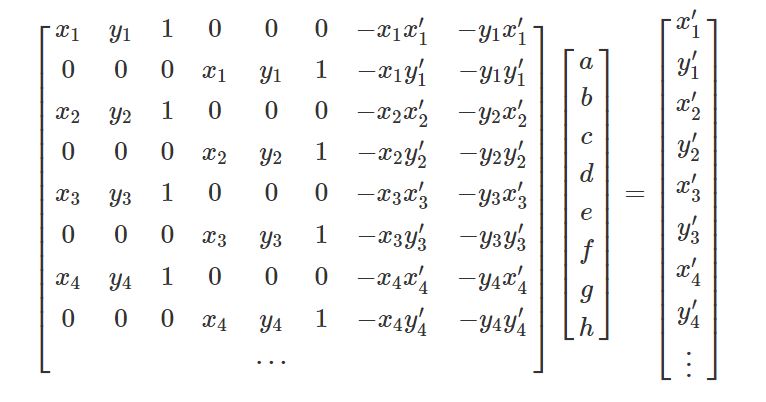
I implemented a method to recover the 3x3 homography matrix by using n-by-2 matrices holding the (x,y) locations of n point correspondences from the two input images. In order to compute the entries in the homography matrix, I set up a linear system of n equations (i.e. a matrix equation of the form Ah=b where h is a vector holding the 8 unknown entries of H). This is described below:
I provided more than 4 correspondences since with only 4 points, the homography recovery will be very unstable and prone to noise. This system could then be solved through least squares as follows:
Point matches were provided with a mouse-clicking interface.
Warp the Images
I warped my images using the parameters of the homography. I implemented a method to use the image to be warped and the homography matrix as inputs to warp the image, while avoiding aliasing when resampling the image. Image warping examples are shown below, where the original warped images used are shown above in the first section titled "Shoot the Pictures":
Warped Image 1: Fancy Building Room
Warped Image 2: Chrysler Building, New York
Warped Image 3: Book
Image Rectification
Below are examples of rectified images. To do this, I took a few sample images with some planar surfaces, and warped them so that the plane is frontal-parallel (e.g. the night street examples above).
Note that since here I only have one image that I need to compute a homography for, say, ground plane rectification (rotating the camera to point downward), I defined the correspondences using what I knew about the image. For example, if I knew that the image is square, I can click on the four corners of that image to be rectified and store them in im1_pts while im2_pts I define by hand to be a square, e.g. [0 0; 0 1; 1 0; 1 1]. After selecting the 4 points on the skewed image, I then used warping to determine a reasonable quadrilateral output region for the unskewed points.
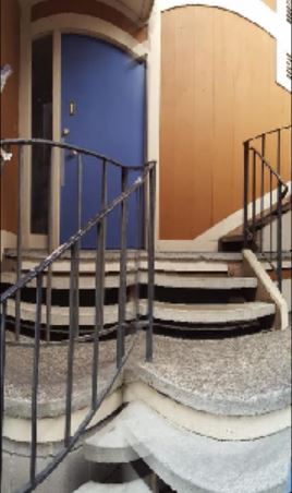
Rectified Image 1: Fancy Building Room
(rectifying the image door)
Rectified Image 2: Chrysler Building, New York
(rectifying the Chrysler Building)
Rectified Image 3: Book
(rectifying the book text)
Blend the Images into a Mosaic
I warped the images so they're registered and created an image mosaic, using weighted averaging. All the images
are warped into a new projection, and are added in one by one, slowly growing the mosaic.
The image size is determined for the final mosaic and then warped into that size. Thus, a stack of images define the mosaic. Next, using weighted averaging, the images were blended together to produce a single image by applying simple feathering (weighted averaging) at every pixel. The pixel at the center of each (unwarped) image is set to 1 and it falls off linearly until it hits 0 at the edges.
Planar Projection (using Weighted Average Blending)
Apartment Uncropped Image
Apartment Cropped Image
Genetics & Plant Biology Building Uncropped Image
Genetics & Plant Biology Building Cropped Image
Trees Uncropped Image
Trees Cropped Image
Bells & Whistles Cylindrical Projection (using Weighted Average Blending) Description:
I used cylindrical mapping to project my mosaic image. This is often a better way to represent
really wide mosaics. I used inverse sampling from the original pre-warped images to make my mosaic the best possible resolution,
while picking a focal length (radius) that looks good.
Apartment Uncropped Image
Apartment Cropped Image
Genetics & Plant Biology Building Uncropped Image
Genetics & Plant Biology Building Cropped Image
Trees Uncropped Image
Trees Cropped Image
Full 360 Degree Cylindrical Projection (using Weighted Average Blending) Description:
Instead of a planar-projection mosaic, I used a cylindrical projection instead. I performed a cylindrical warp on all my input images (Bancroft Library) and stitched them together using translation only to produce a full 360 degree panorama.
Bancroft Library Uncropped Image
Bancroft Library Cropped Image
What I Learned:
Implementing homography can be tricky, but it has many interesting applications for smoothly stitching images togther.
I finally have a better understanding as to how image mosaics and panoramas are formed.
Project 6B: Feature Matching and Autostitching
The goal of this project is to create a system for automatically stitching images into a mosaic. A secondary goal is to learn how to read and implement a research paper. The project will consist of the following steps:
1. Detecting corner features in an image (Using the Harris Detector)
2. Extracting a Feature Descriptor for each feature point
3. Matching these feature descriptors between two images
4. Use a robust method (RANSAC) to compute a homography
5. Proceed to produce a mosaic showing 3 both manually and automatically stitched results side by side
Detecting corner features in an image (Harris Detector)
Using the Harris Corner Detection algorithm, measure a close match to a windowed function.This determines
whether or not there is a corner in this image vicinity, which tells us where the corner(s) is located.
It is more helpful to detect corners than edges because it would give us feature points without having fixed
image corners. Below are the original images examples:
Apartment Left Image Original
Apartment Right Image Original
Bancroft Library View 1 Image Original
Bancroft Library View 2 Image Original
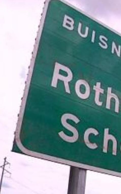
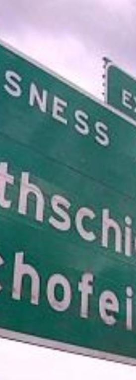
Sign Left Image Original
Sign Right Image Original
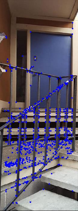
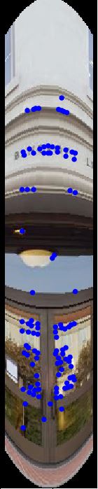
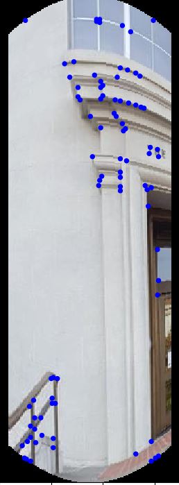
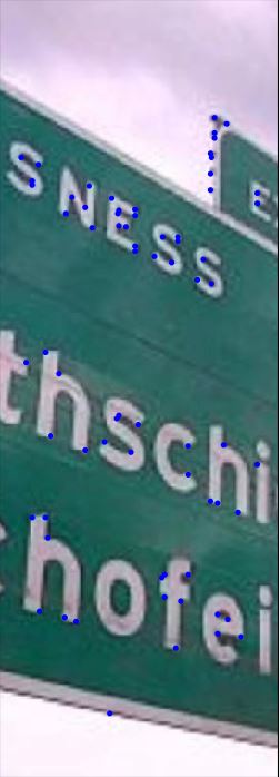
With Harris Detector Points
Apartment Left Harris Detector Points
Apartment Right Harris Detector Points
Bancroft Left Harris Detector Points
Bancroft Right Harris Detector Points
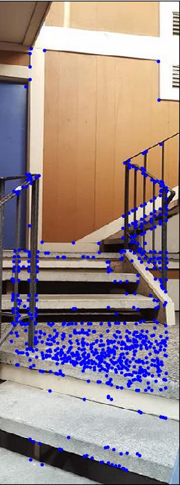
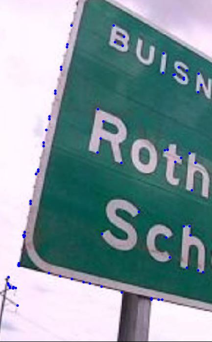
Sign Left Harris Detector Points
Sign Right Harris Detector Points
Adaptive Non-Maximal Suppression
The MOPS paper describes adaptive non-maximal suppression for the harris detector algorithm's corners. We want to extract fewer points because the computation cost of matching is superlinear in the number of interest points. To get correspondences between the images, points should be distributed over the complete image. For every point, find the minimum radius to the next feature point such that the corner response for the existing interest point is less than some constant multiplied by the response for the other point. Then, the algorithm will choose the interest points with the
greatest radius to next prominent feature point. This will ensure that we are
retaining points with the strongest responses that are also far away from other strong points, and thus giving points nicely distributed. Below are image examples:
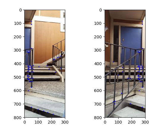
Apartment Adaptive Non-Maximal Suppression
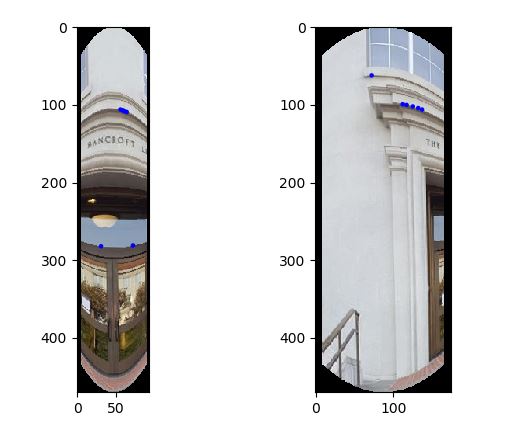
Bancroft Adaptive Non-Maximal Suppression
Sign Adaptive Non-Maximal Suppression
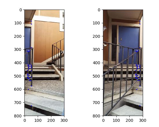
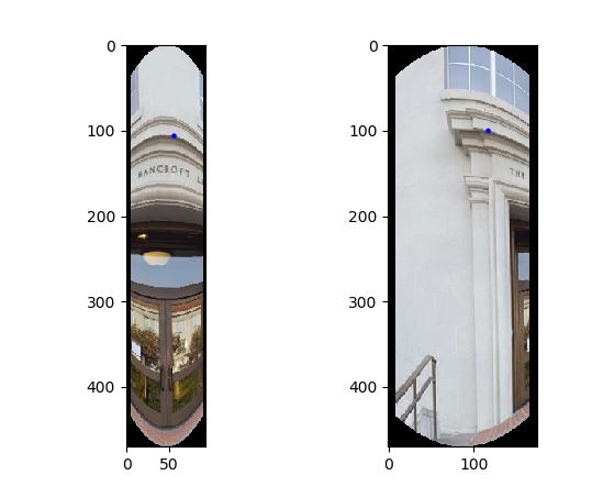
Extracting Features and Feature Matching
In order to now find the square N by N feature patches in the image,
the algorithm is designed to look at 40x40 interest points, and then it downsamples these patches to be of size 8x8.
Downsampling helps because it removes the high frequency signal that interferes with the accurate matching of features, as it is low-pass filtering the image. This is good because it prevents noise from interfering with the general feature that that is to be matched.
Then, we normalize the patches through mean subtraction and standard deviation division, thereby producing features that are invariant to overall intensity differences and to the shift in RGB distribution.
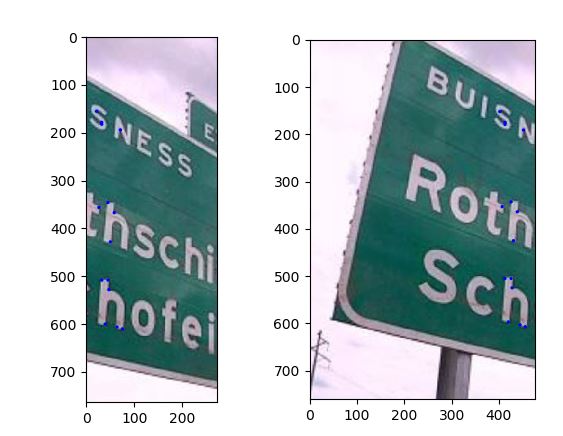
After the features are normalized and now contain the invariant properties, SSD is used to match the features alongside the other features. Lastly, a ratio scaling is computed between the best and second best feature detected, which allows us to pick only those matches that have a single good match as opposed to multiple matches. Matches that satisfy the ratio computed are returned. Below are the points returned by the algorithm as well as the corresponding pixel intensities visualizations.
Apartment Extracting Features & Matching
Apartment Left (Left), Apartment Right (Right)
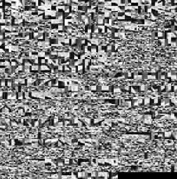
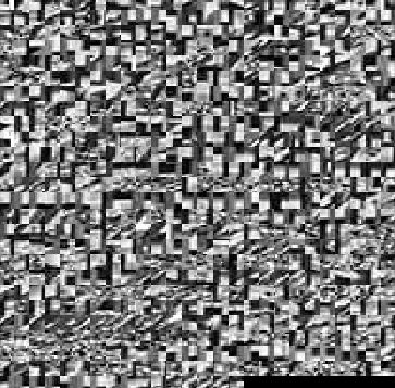
Apartment Left Feature Descriptor Pixel Intensity Visualization
Apartment Right Feature Descriptor Pixel Intensity Visualization
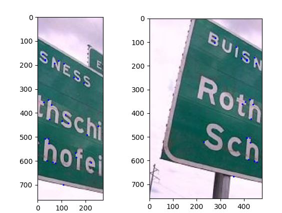
Sign Left Feature Descriptor Pixel Intensity Visualization
Sign Right Feature Descriptor Pixel Intensity Visualization
The RANSAC Algorithm
After computing the feature matches as described above, note that there may still be outlier matches in the set.
To fix this, we use as an estimation technique the RANSAC algorithm. This is done by choosing 4 points and
computing a homography of those points. Then, we find the inlier point number using the homography calculation
that we previously computed and use the largest homography set found. Eventually, the RANSAC algorithm will find the
right homography point set of inliers to use. Lastly, the new homography is computed using this largest set.
Auto-stitched Mosaics
Below are the automatically stitched multi-image panorama examples. I played around with both
automatic stitching using the planar projection and cylindrical projection separately, as sometimes
one projection gave a better visual stitching results than the other projection. Below are examples
of stitching with the image manually, and autostitching of the images with the type of projection used
indicated.
Automatic stitching image of: Apartment
Using the Planar Projection Technique
Manual stitching image of: Apartment
Using the Planar Projection Technique
Automatic stitching image of: Bancroft
Using the Cylindrical Projection Technique
Manual stitching image of: Bancroft
Using the Cylindrical Projection Technique
Automatic stitching image of: Sign
Using the Planar Projection Technique
Manual stitching image of: Sign
Using the Planar Projection Technique
Reading the MOPS paper was very enjoyable. The Harris Detector algorithm and the RANSAC algorithms were
very interesting. In addition, I learned that there is no one right projection that can be used to produce
the best images. Often, different projections (ie. planar or cylindrical) should be tried out to see
what produces good images.
Given an unordered set of images, some of which might form panoramas, I automatically discover and stitch these panoramas. Upon stitching the panoramas, a threshold of feature detected inlier
corresponding points is found, and only if this exceeds the threshold are the images stitched together. This
method thereby stitches images together via parorama recognition. Below are the results.