Overview

A single image inherently has limitations on how large a scene can be captured; however, when we mosaic, or stitch, many images together, we can create a larger field of view. The challenge is, how do we stitch the images together so they are nicely aligned?

It is not enough to simply overlap and blend two images together, even though there are features shared across the images. We will visit the use of projective transformations to warp an image into the same plane as the other, provided the two images shared the same point of projection (i.e. the camera didn't translate between shots). Finally, how do we blend the images together into one cohesive image? We will attempt to create our own panoramas in this project.

Starting Images

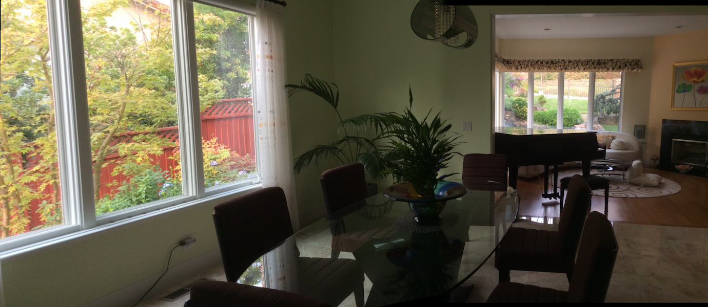
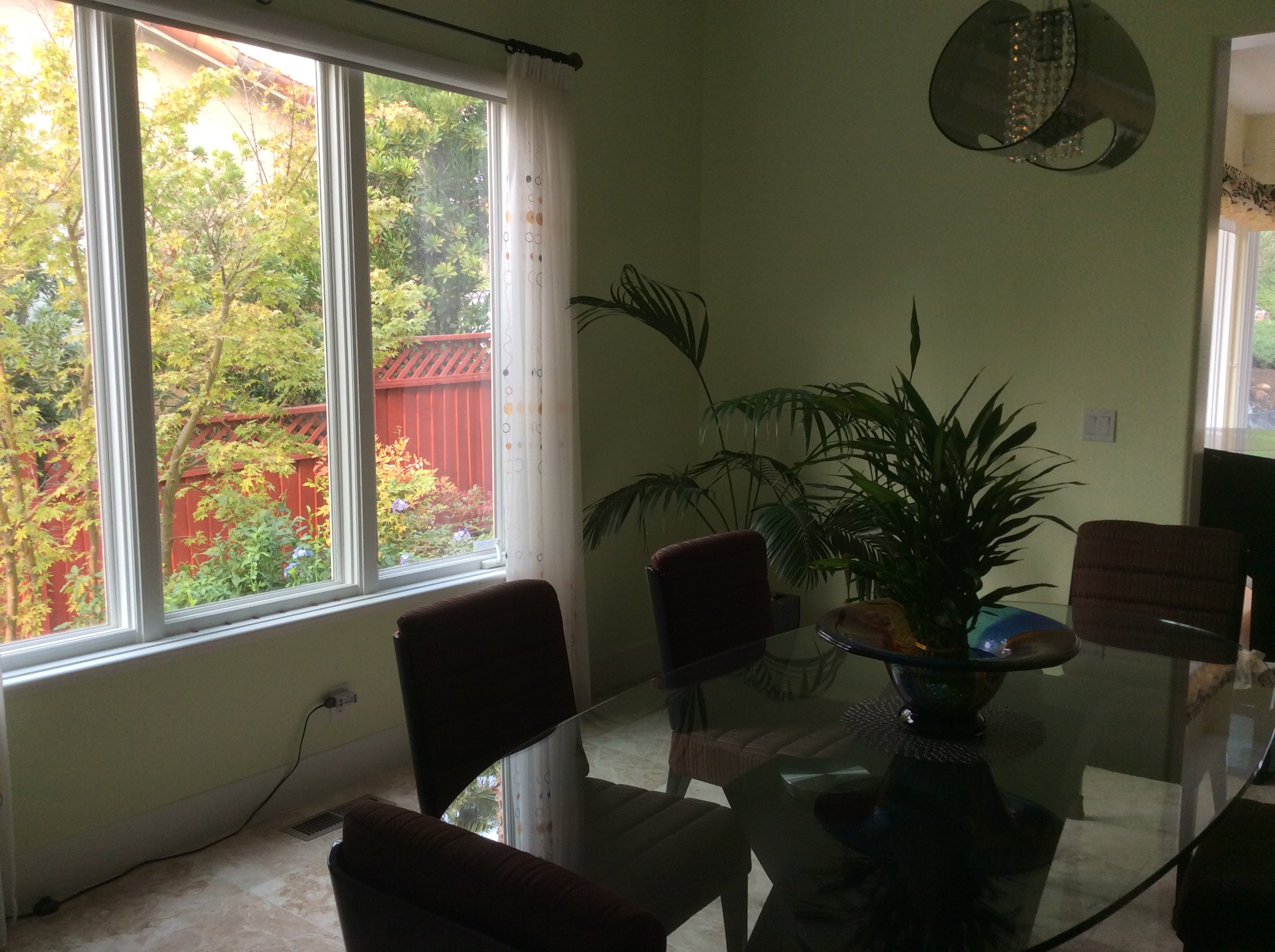
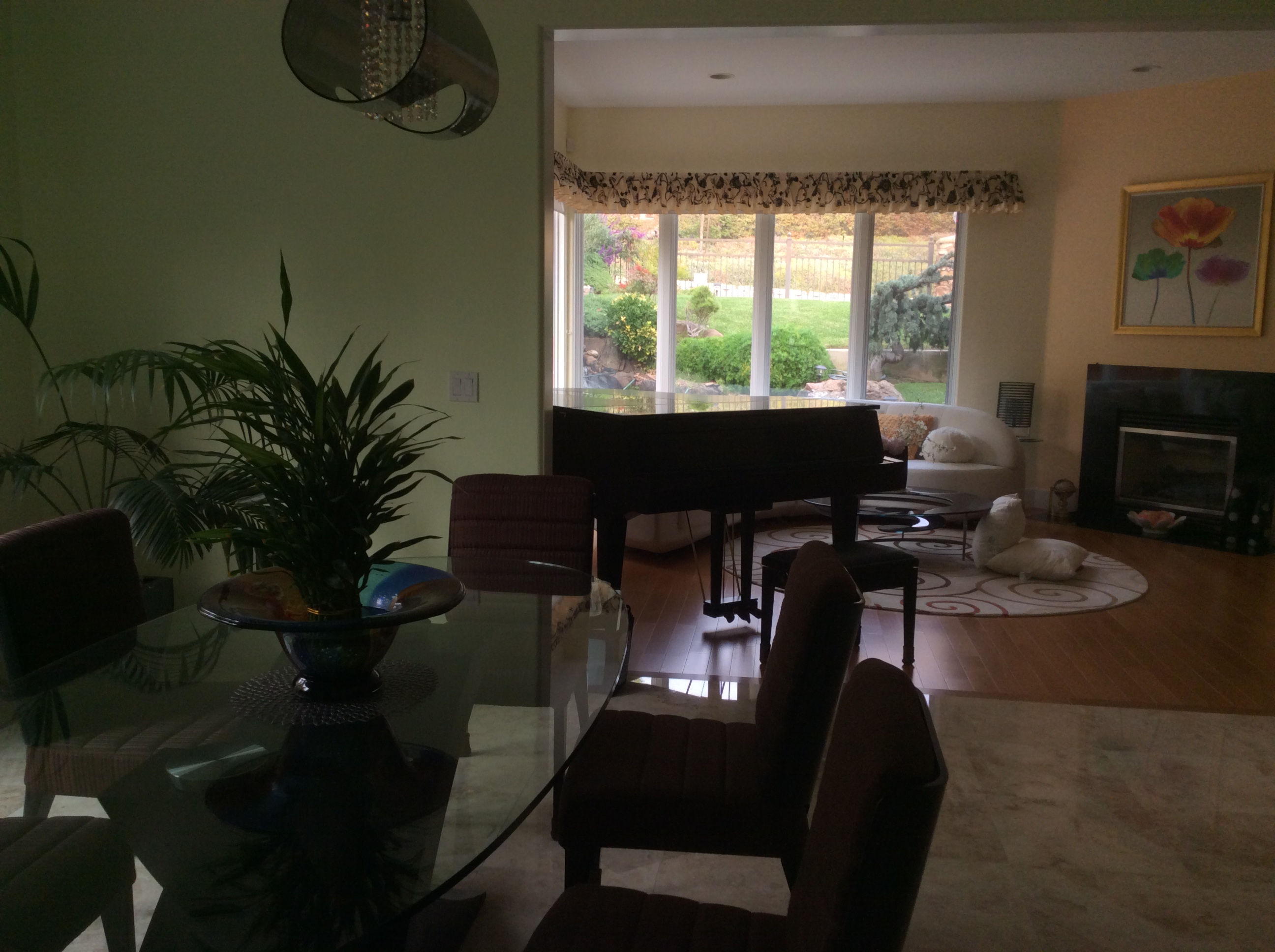
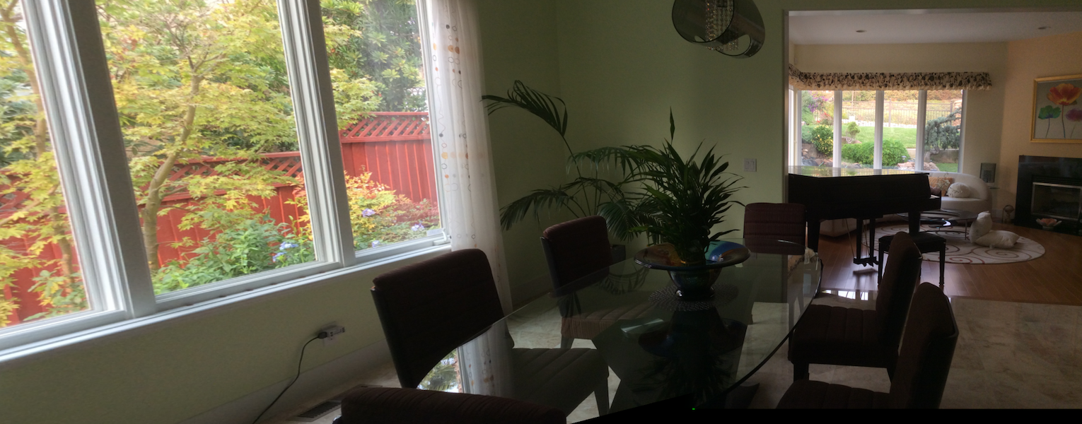
First Set

First Set

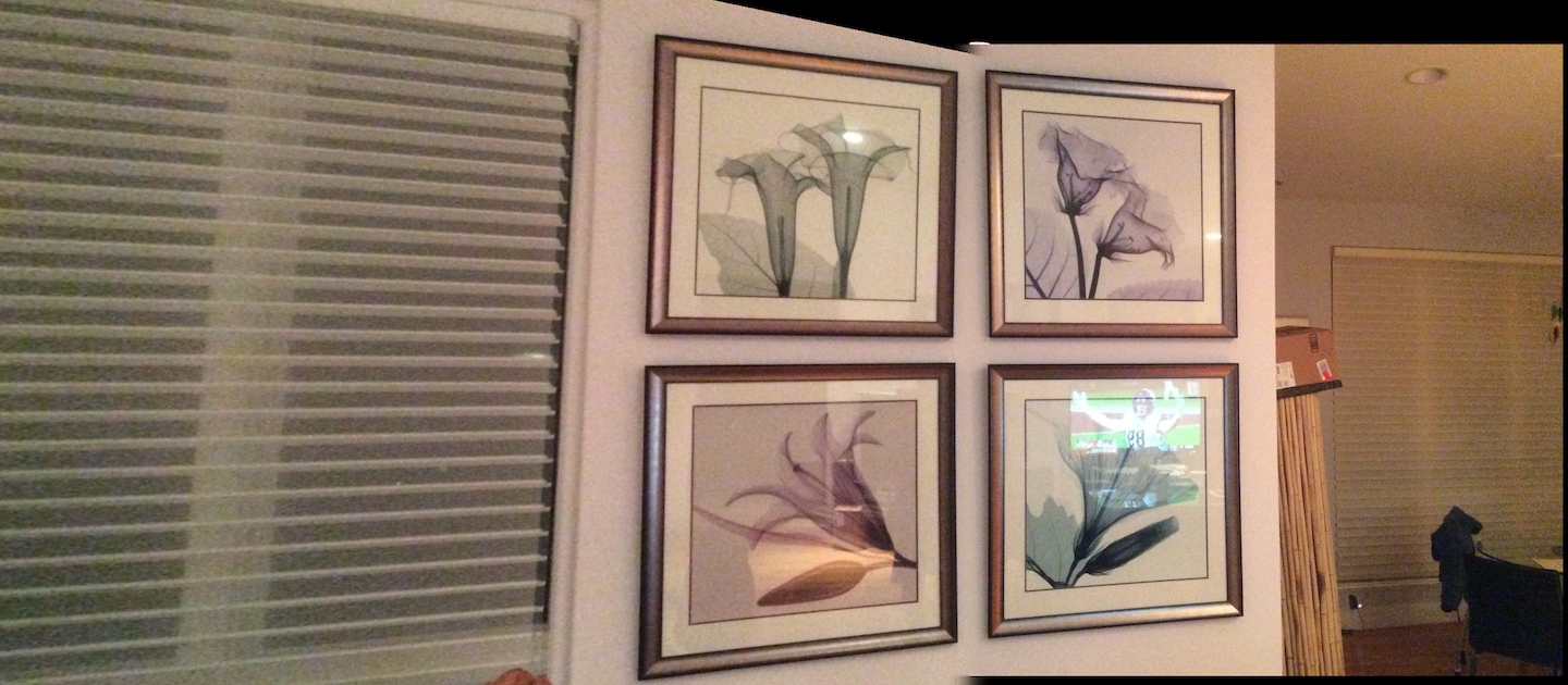
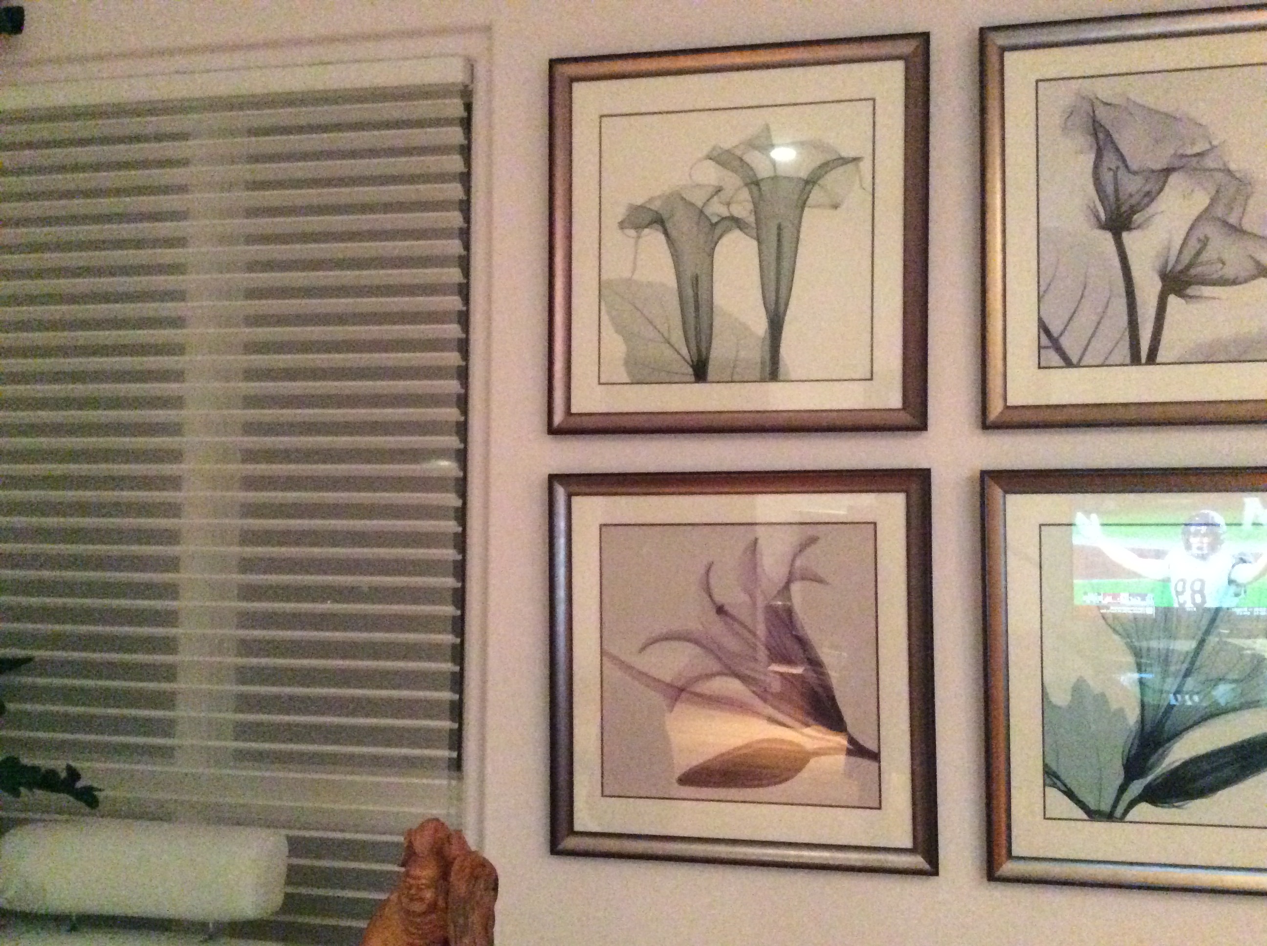
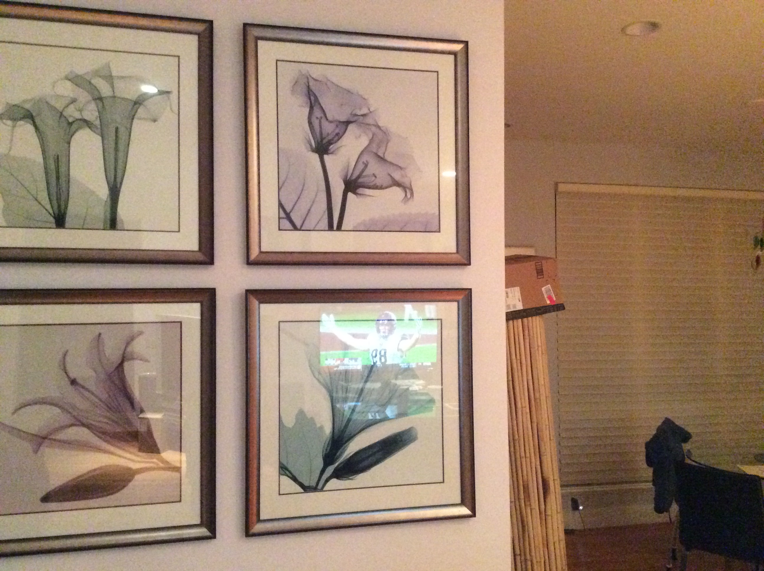
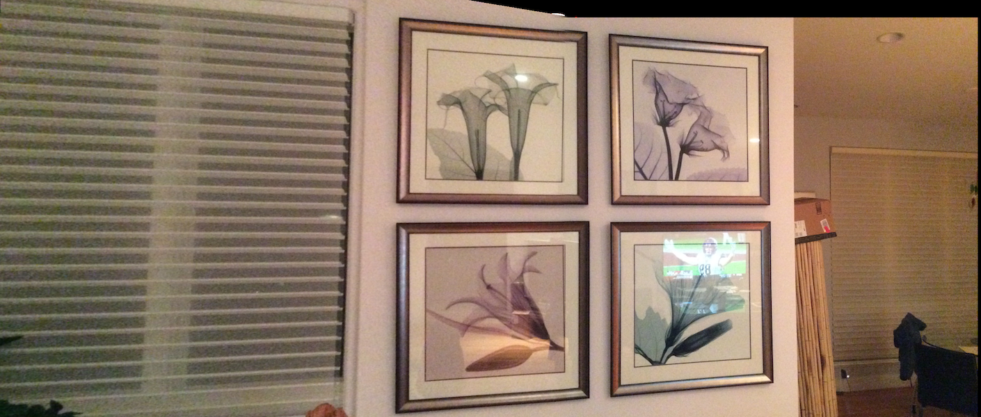
Second Set

Second Set

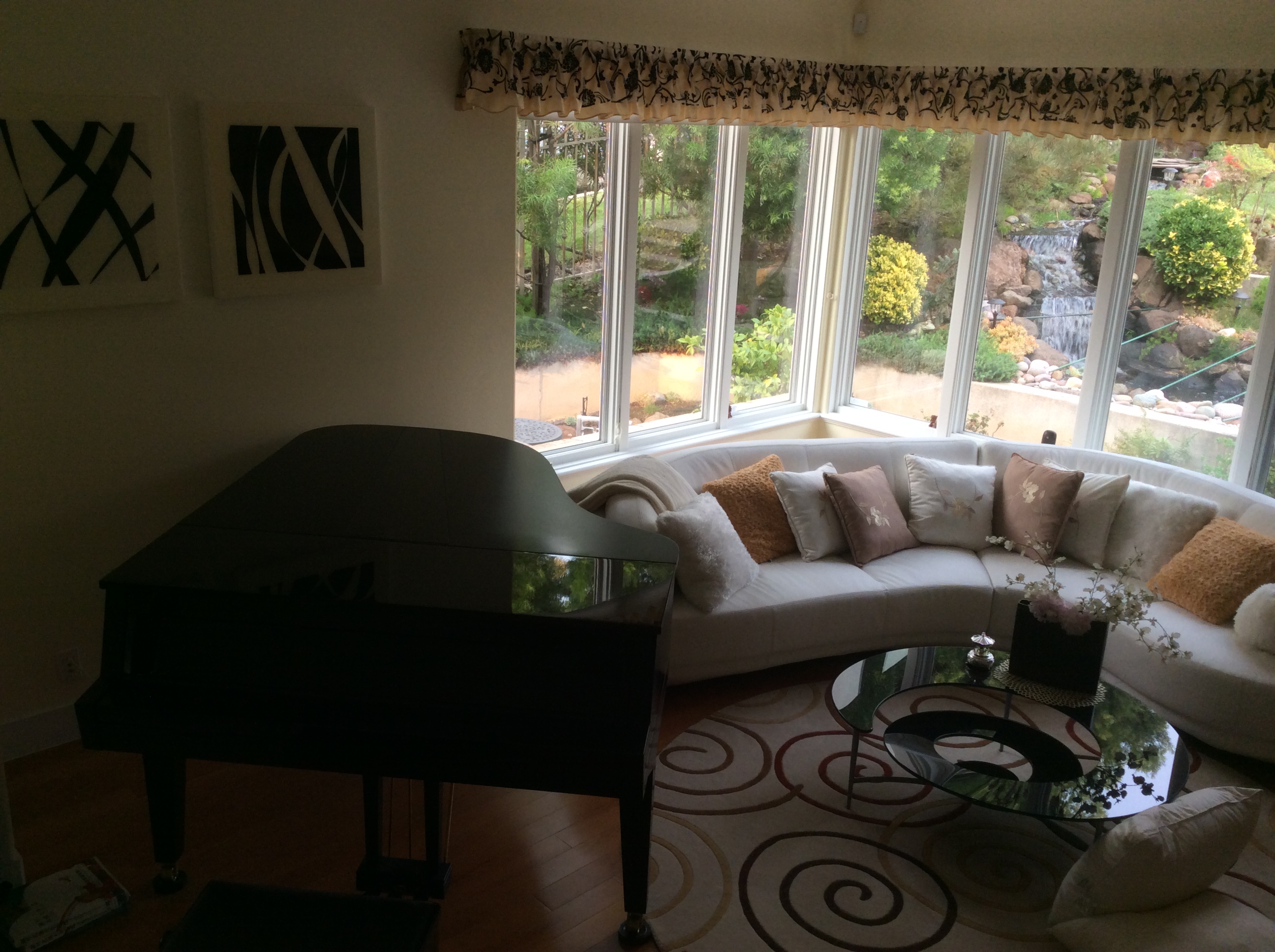
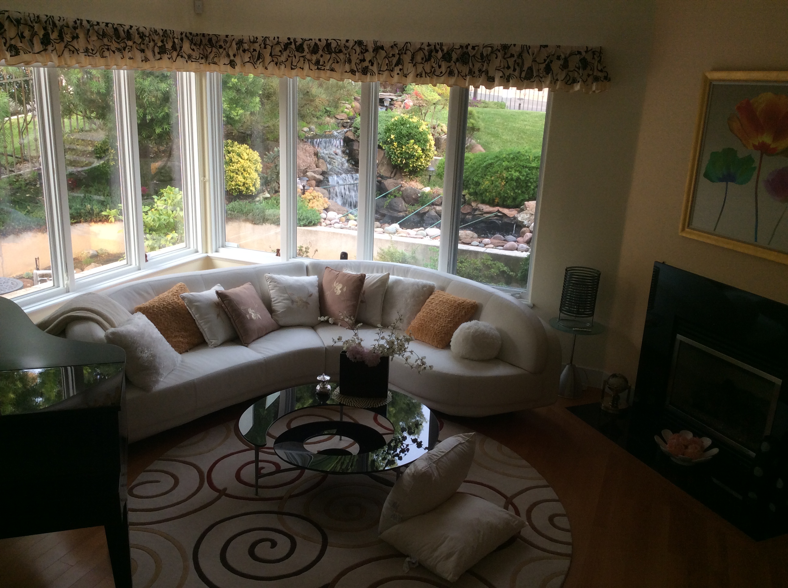
Third Set

Third Set

Homography, Warping, and Image Rectification

We compute the homography between 2 images using the equation p’=Hp, where H is a 3x3 matrix with 8 degrees of freedom (we set the lower right corner, the scaling factor, to 1). p and p' are vectors of corresponding points.

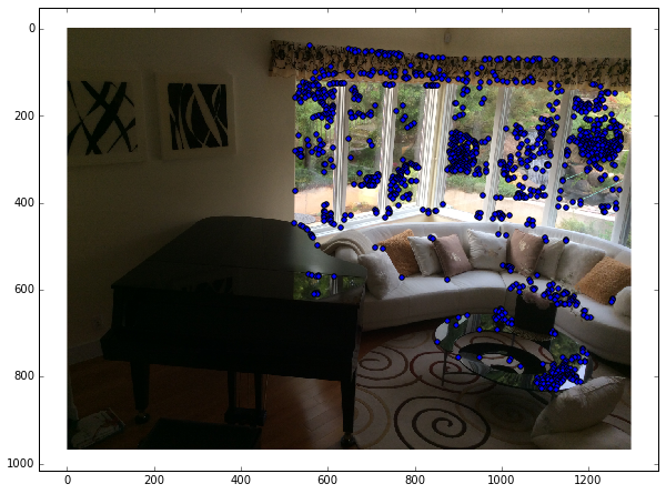
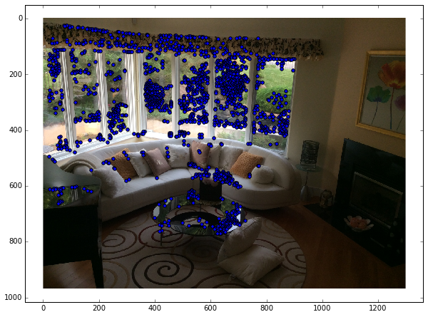
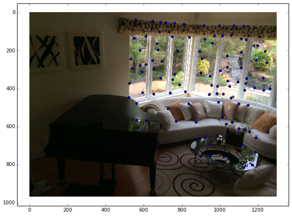
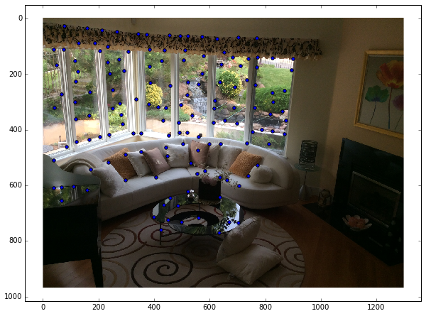
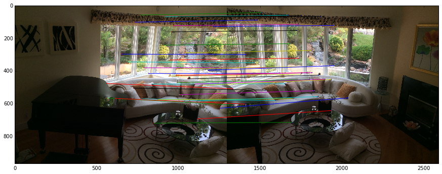
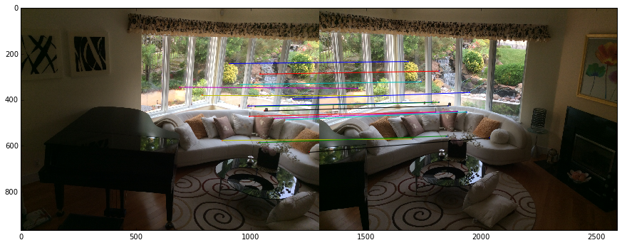
We first click on corresponding points in the two photos, to get these lists of correspondences (need at least 4 (x, y) correspondences to compute 8 degress of freedom). Then, we can compute the transformation matrix between the two images: H.

Once we compute the transformation, we can warp all of image1 to align with image2 (or vice versa). Since H defines the transformation, we apply H (using inverse warping preferably), to transform our image into the desired shape.

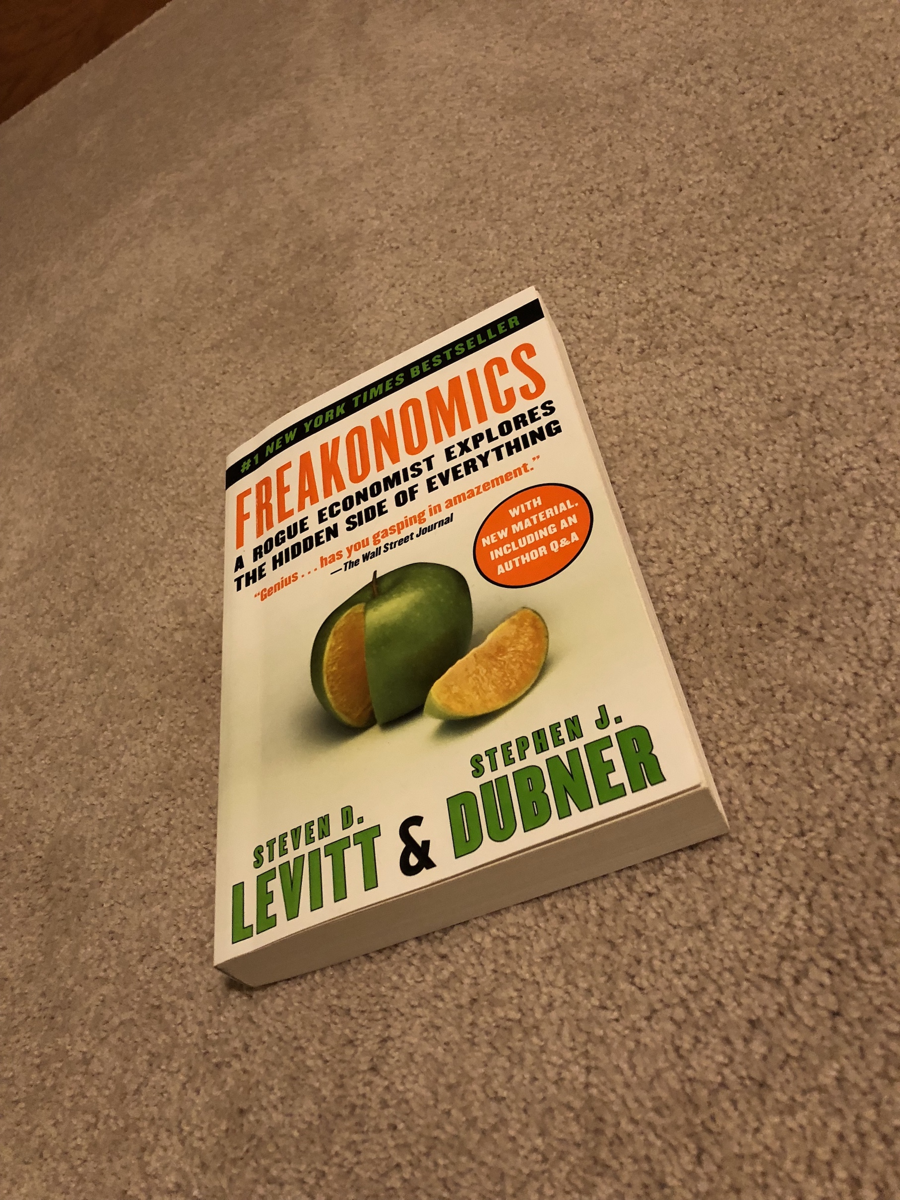
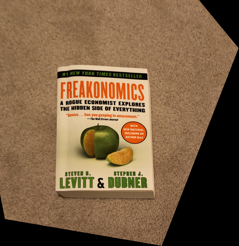
Below are two examples of image rectification. I took two photos of two books at angles such that they were not rectangular. Next, I selected the four corners of each book and manually set their corresponding points to be corners of a rectified rectangle. Using the computed homography from these correspondences, I warped the original image into tthe rectangle. You can see that the results are the books as if viewed top down from above. (Like the PDF scanner apps on our phones!)

Original Image

Rectified Image

Original Image

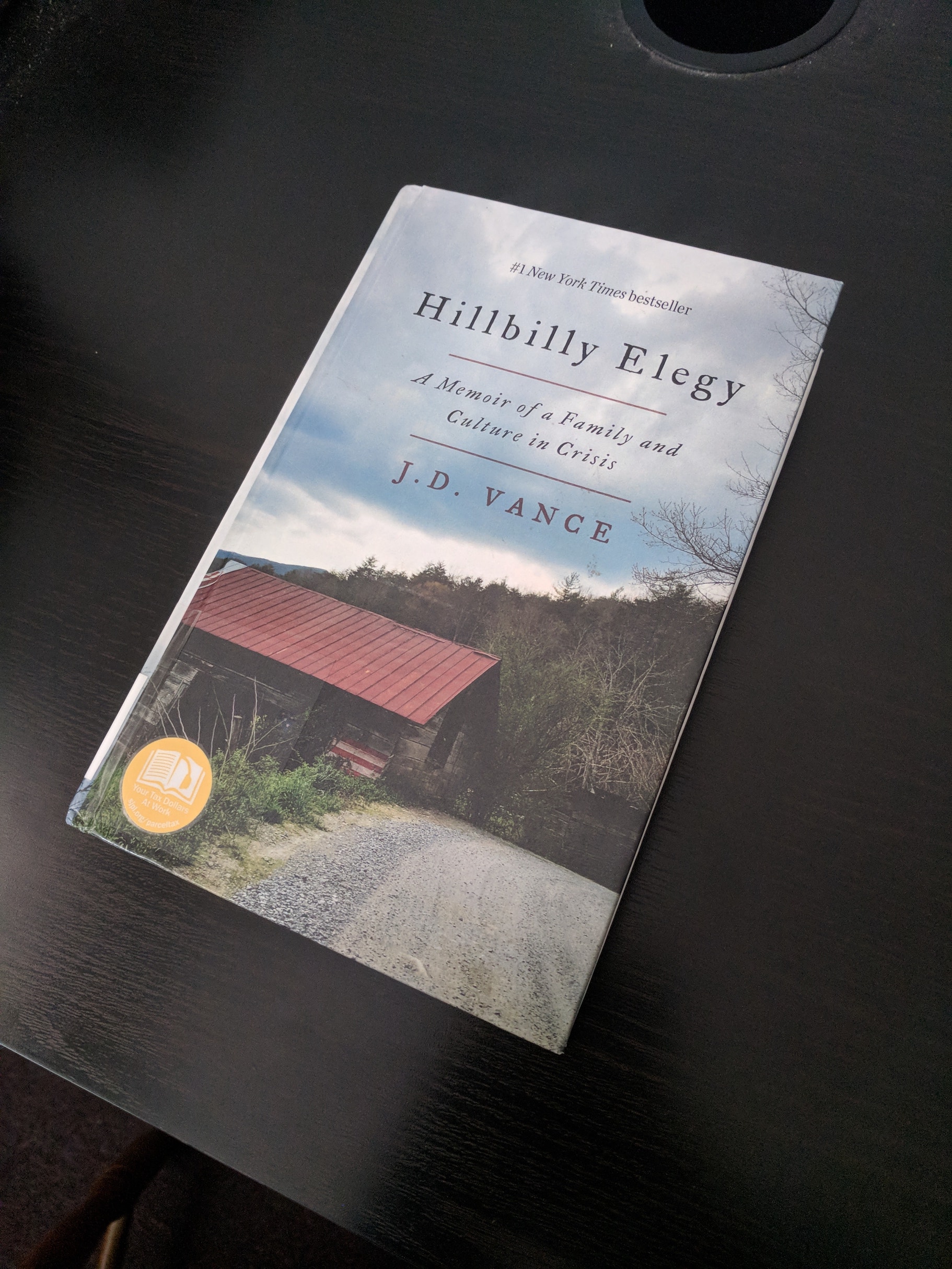
Rectified Image

Creating Mosaics

For each pair of images above, I first expanded the images through np.pad to get a final output image size. I clicked on correspondences, from which I computed the projective transformations. Then, I warped one image to align nicely with the other.

Then, to blend the two images together, in order to avoid strong visible edges, I used Laplacian blending (2-band/3-band) from proj3. I used a linear mask to specify how much of each image I wanted in each region, then used this mask and Gaussian and Laplacian stacks to smoothly blend the two images.

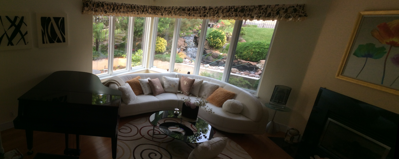
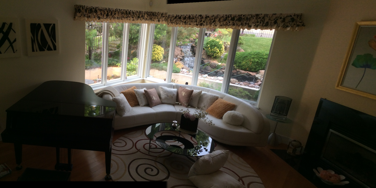
Here are the resulting cropped mosaics (click to enlarge):

First Set

Second Set

Third Set

There may be some seam artifacts, which I believe to be due to two main possibilities: shift in center of projection and quality of correspondences.

Manually clicking on correspondences with the ginput tool is not the most accurate, and when there's a lot of little detail in the images to match up, little errors can be quite visible.

Summary

I think this part is pretty cool and makes me appreciate the panorama tool on my phone! I have definitely shifted the COP on many panoramas taken on my phone and they still turn out to look great. Image rectification and homography is a cool idea especially when applied, and being able to "shift" the camera after taking a photo is a nifty idea. It's almost magical! Especially with the pretty simple idea of warping.

Overview

Part B is an improvement to part A, as we continue to create our own panoramas. In part A, the feature points in each image had to be chosen manually by the user. In this part of the project, correspondences will be automatically selected and matched to allow for effortless panorama stiching. The starting image sets are the same as those in Part A above.

Step 1. Detecting Harris corner features

We choose corners for our possible corresponding feature points, because corners are prominent and easily recognizable across different images of the same setting. Shifting a small window in any direction around a corner should give large change in intensity, i.e intensity changes a lot around corners.

To detect corners automatically, we use the Harris Corner Detection algorithm. Harris Corners have several desirable properties, including rotational invariance and partial invariance to affine intensity change. Resulting corners shown below (click to enlarge):

First Set All Harris Corners

First Set All Harris Corners

Furthermore, we want the best features distributed evenly across each image, for a more robust homography matrix that transforms the whole image well. Therefore, we run Adaptive Non-Maximal Suppression on our Harris corners: choosing corners that are the "best" corner in their neighborhood (within a radius r). ANMS takes into account strongest points as well as the distance from previous points.

For each point, the minimum distance to another point with a response value that is still greater than its own after being reduced by a scale factor is found. If a point has a large corresponding radius, it is far from other points that have a much larger response value, and thus it is a good local max. Below are results with ANMS applied. As you can see, the points are much more evenly spaced out.

First Set ANMS Harris Corners

First Set ANMS Harris Corners

Step 2: Extracting Feature Descriptors

Now that we have our corner features, we need to prepare for matching features across images. Therefore, we need to extract image patches around each feature. Each patch is an 8x8 patch of pixels sampled from a 40x40 patch around the corresponding feature.By sampling the pixels at a lower frequency than the one at which the interest points are located (higher pyramid level), patches are less sensitive to the exact feature location. Each feature patch was then bias/gain normalized, to lessen the effects of overall intensity differences and distribution of RGB. Below are some sample 8x8 feature patches.

Sample 8x8 Feature Patches

Step 3: Matching feature descriptors between two images

To match features across images, we compute the distance between descriptors. Each patch in the first image is compared to all in the second, with the distance between patches given by the sum of squared differences (SSD) formula. In essence, for each patch in image 1, we find the closest match in image 2, i.e. with the lowest SSD.

But note: only the overlapping features should get matched! And with noise being present, feature space outlier rejection is needed. Incorrect matches can also have low distances, and simple thresholding on the distance is not the best procedure. Therefore, we use the "Russian Granny trick”; we only consider that feature and its nearest neighbor in the other image to be a match where the ratio of the 1-NN dist / 2-NN dist were lower than a certain threshold. This chosen Lowe's ratio threshold was 0.6. (Credit to Lowe!)

Below are the 36 matches/correspondences found before RANSAC: (click to enlarge)

Feature matching without RANSAC (36 Correspondences)

Step 4: Computing Homography with RANSAC

As seen above, we still have some outlier matches, which would greatly affect the homography. Therefore, the next step is to use the Random Sample Consensus (RANSAC) algorithm to recover the best possible homography from the matched interest points.

We use 4-point RANSAC: choose 4 correspondences at random, compute the exact homography, then apply this homography to every one of our matches. If the error between the transformed point and the match is small (within a low epsilon), that correspondence is considered an inlier. We repeat this process for several thousands of iterations, and retain the largest set of inliers. Finally, we use this largest inlier set to compute a robust homography to warp one image to the other's perspective.

Below are the 15 correspondences found after RANSAC: (click to enlarge)

Feature matching with RANSAC (15 Correspondences)

Step 5: Laplacian Blending to Create Mosaic

Using the final homography computed from RANSAC, one image is warped to align with the other. Blending was the same as in part A.In order to avoid strong visible edges, I used Laplacian blending (2-band/3-band) from proj3. I used a linear mask to specify how much of each image I wanted in each region, then used this mask and Gaussian and Laplacian stacks to smoothly blend the two images.

Below are the manual results from part A and automatic results from part B side by side.

Manual First Set

Auto First Set

Manual Second Set

Auto Second Set

Manual Third Set

Auto Third Set

Summary

RANSAC and the Lowe's ratio were very cool, and I agree with Professor Efros that RANSAC is “one of the best algorithms in computer vision in the last 40 years. So simple, works amazing”. Much respect to panorama software on our phones that do it so seamlessly and efficiently too!