CS194-26 Project 6A: AutoStitching Photo Mosaics
Josh Zeitsoff, cs194-26-abi
Overview
Our goal is to create a photo mosaic by taking multiple pictures that have some overlap, warping one image towards the other, and blending them together to form a mosaic.
Rectified Images
For each image, I chose the corner points of the sign, determined correspondence points of my desired output image (which was a square), and warped the image towards those correspondence points. This was done by determining the H matrix and applying an inverse warp to each pixel in the output image, using interpolation to determine pixel values from the original image.
Original Image

Rectified Image

Original Image
Rectified Image
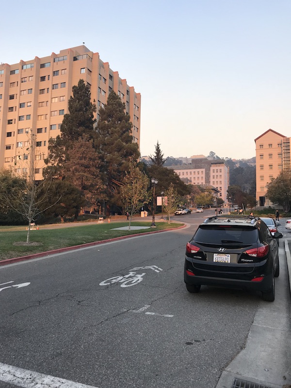
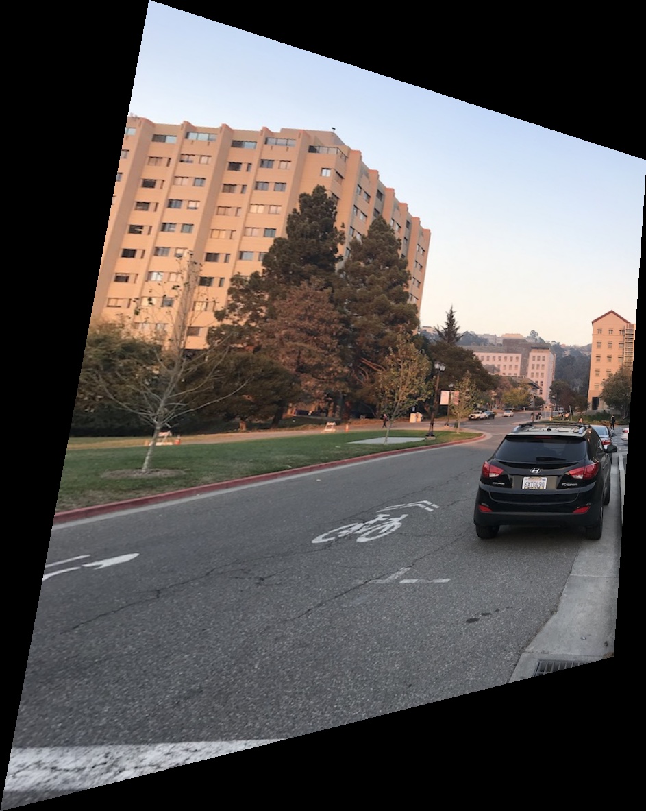
Warped Images
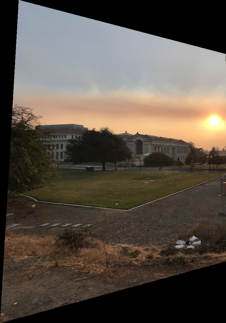
For each image, I first chose 8 points from the left image and 8 points from the right image to use in determining the H matrix. Once I had done so, I warped the left image towards the right. I determined the shape of the warped image by seeing how the H matrix transformed the corners of my original image, and went through each pixel coordinate in the output image. For each of these coordinates, I applied an inverse warp and used interpolation to find the pixel values from the original image. One thing to note are the parts of the warped image where the inverse warp resulted in a pixel coordinate out of bounds of the original image. You can see this where the blended image has pixels with no value, which are black.
Left Image
Left Warped towards Right
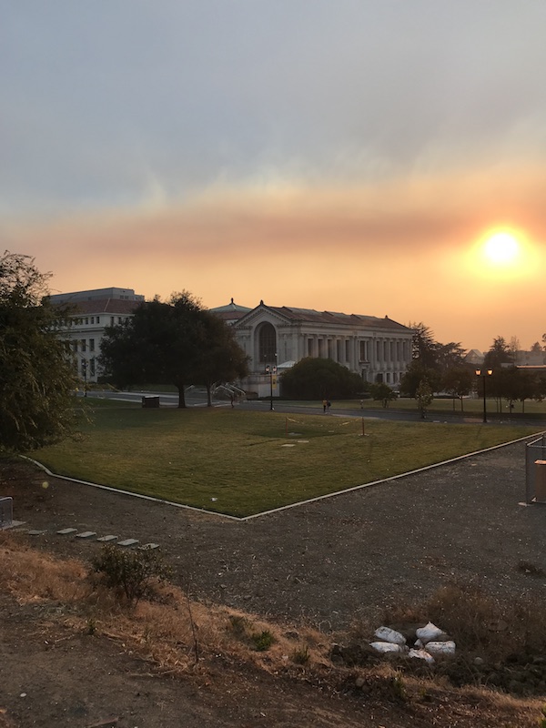
Right Image
Left Image
Left Warped towards Right
Right Image
Left Image
Left Warped towards Right
Right Image
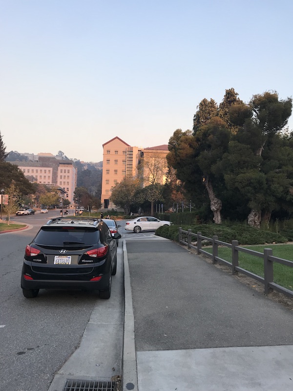
Blended Images
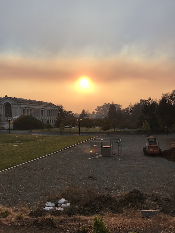
Now that I had a warped left image, I needed to first align it with the right image for it to be blended. To align the 2 images, I chose the same point in each image (for example, the same corner of the same building) and found the column and row offset from this point in each image. This gave me the desired effect of aligning the 2 images on top of each other, albeit with a line where the 2 images met. Once the 2 images were aligned, I used alpha blending (with alpha = the distance transform of each image) to blend the 2 images together.
Warped Left Image
Right Image
Blended Image
Warped Left Image
Right Image
Blended Image
Warped Left Image
Right Image
Blended Image
What I learned about stiching and mosaics
Changing the POV of an image through warping is pretty cool, and you can change the shape of objects in images. One thing I had to account for was that either of the 2 shapes could be irregular - we are able to take a sign that, given the perspective, is a trapezoid, and warp it into a square. Likewise, our transformation could turn a square image into an irregular one, which required some extra processing to determine the boundaries of the output shape.
CS194-26 Project 6B: AutoStitching Photo Mosaics
Overview
The goal of this project was to automatically detect correspondence points in the two images, and use these to warp them instead of manually selecting correspondence points as we did in 6A.
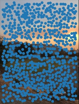
Harris Interest Points
As we found in project 6A, the best correspondence points tend to be corners that we can easily match between 2 images. One way to detect corners in an image is to use the Harris Corner Detection algorithm, which looks at pixels that have significant intensity changes in all directions around them. Below, I used the harris corner starter code and overlaid the points on the original image.
Original Image
Harris Corners
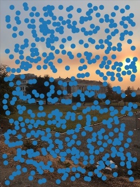
Adaptive Non-Maximal Suppression
To filter these Harris Corners, we apply Adaptive Non-Maximal Suppression. Our goal is to narrow down these corners to better ones, as well as ensure that the corners are spread out throughout the image. We do so by only picking those corners who are a maximum in their neighborhood of r pixels based on their corner strength. We do so by finding the distance, d, from a pixel x_i to the nearest other pixel x_j such that f(x_i) < .9 * f(x_j) , where f is the corner strength function and .9 is chosen as a measure of robustness. For each corner, we now have a value that represents the radius in which this pixel is the maximum. To pick the best 500 corners, we select the 500 pixels with the largest such radii. Below, you can see that the corners are more evenly distributed over the image.
Harris Corners
ANMS Corners
Feature Extraction and Matching
Now that we have a set of 500 corners, we want to come up with a feature descriptor for each corner. We do so by looking at a 40x40 region around each corner and subsampling this into an 8x8 matrix of pixels, remembering to bias/gain normalize by subtracting the mean and dividing by the standard deviation. We'll use these features to attempt to find matching corners from 2 images. To extract our features, we start by going through all features in the first image. For each feature, we find the sum of squared differences between the feature in image 1 and each feature in image 2. We take the nearest neighbor (1-NN) and second nearest neighbor (2-NN) from the set of features in image 2. To remove outliers, we only keep features where (1-NN / 2-NN) < .6 , where .6 was the threshold as determined from the research paper. The idea is that if our 1-NN had some SSD score A , and our 2-NN had some SSD score B , we want points such that A is much smaller than B, meaning our 1-NN is a much better match than our 2-NN and thus more likely to be the feature in image 2 that matches our feature in image 1.
ANMS Corners
Feature Corners
Ransac Corners
Now that we have a set of "matching" features, we still need to narrow these down to correspondence points to use for our homography. We use 4-point RANSAC (RANdom SAmple Consensus) as described in class. Given our 2 sets of feature points (1 set for image 1, one set for image 2), we take 4 random feature points from set 1 and find the matching feature points from set 2 and compute our homography H. We apply H to every feature in set 1, and compute the SSD with the matching feature in set 2. We keep a set of inliers where the SSD is less than some threshold, say .5. We repeat this process, randomly selecting 4 feature points, for a large number of iterations, and keep the largest set of inliers. As you can see below, pre-RANSAC we have some feature points that will result in incorrect homographies, for example those to the left of the left image above the tree. These have no correspondence points in image 2 (which we verify visually) yet according to feature extraction they had some match. RANSAC filters these out, and we can see in the second set of images below.
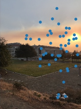
Feature Corners Left Glade
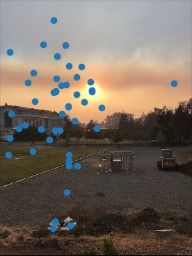
Feature Corners Right Glade
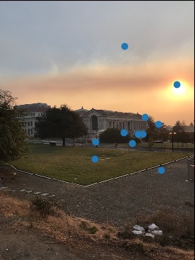
Ransac Corners Left Glade
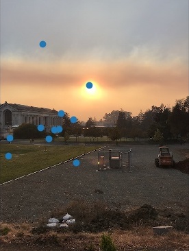
Ransac Corners Right Glade
Correspondence Points
Ransac Corners Left Glade
Ransac Corners Right Glade
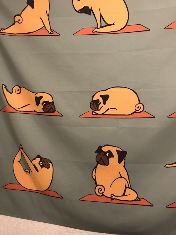
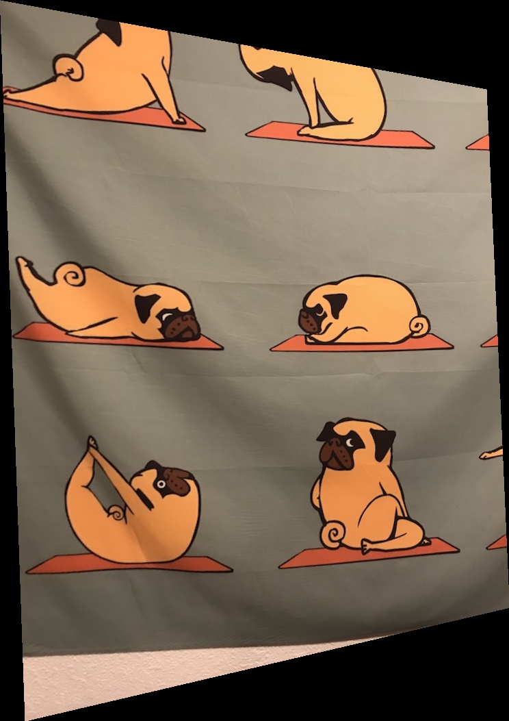
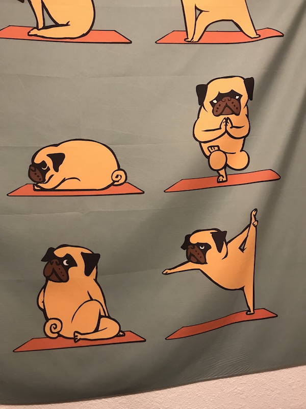
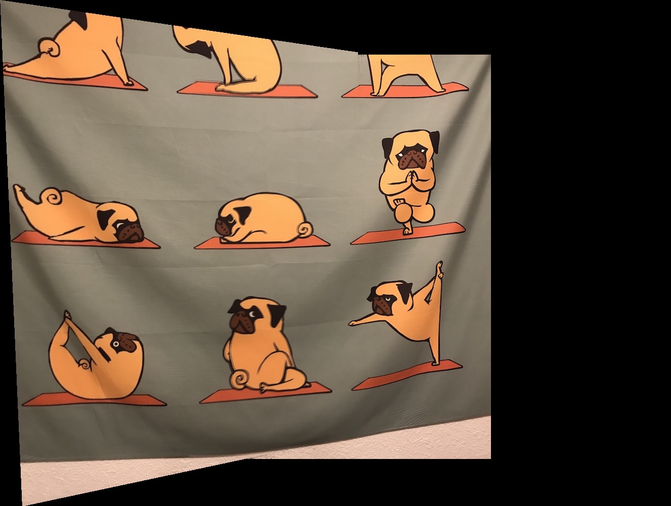
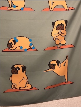
Ransac Corners Left Pug
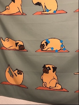
Ransac Corners Right Pug
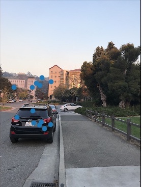
Ransac Corners Left Car
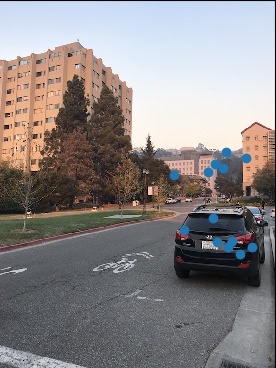
Ransac Corners Right car
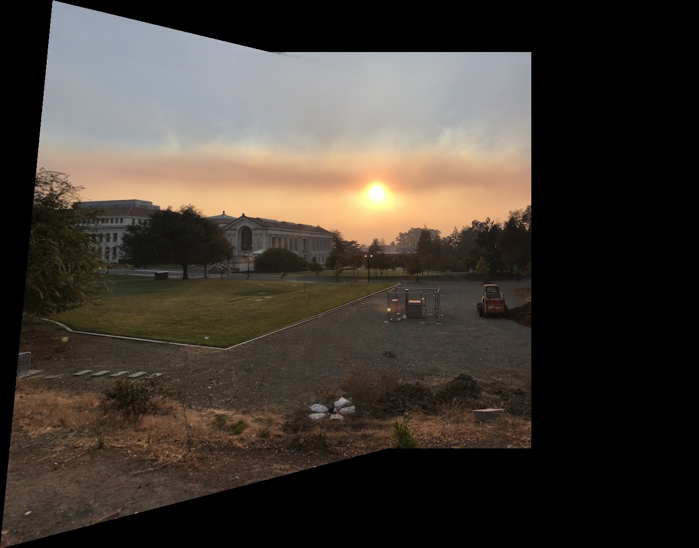
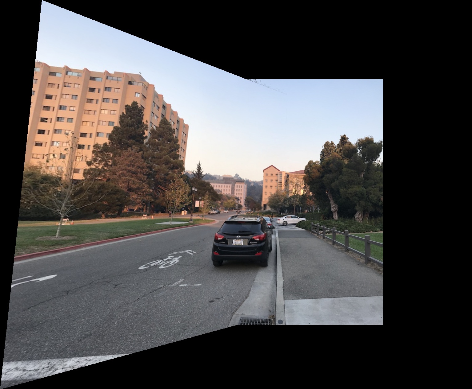
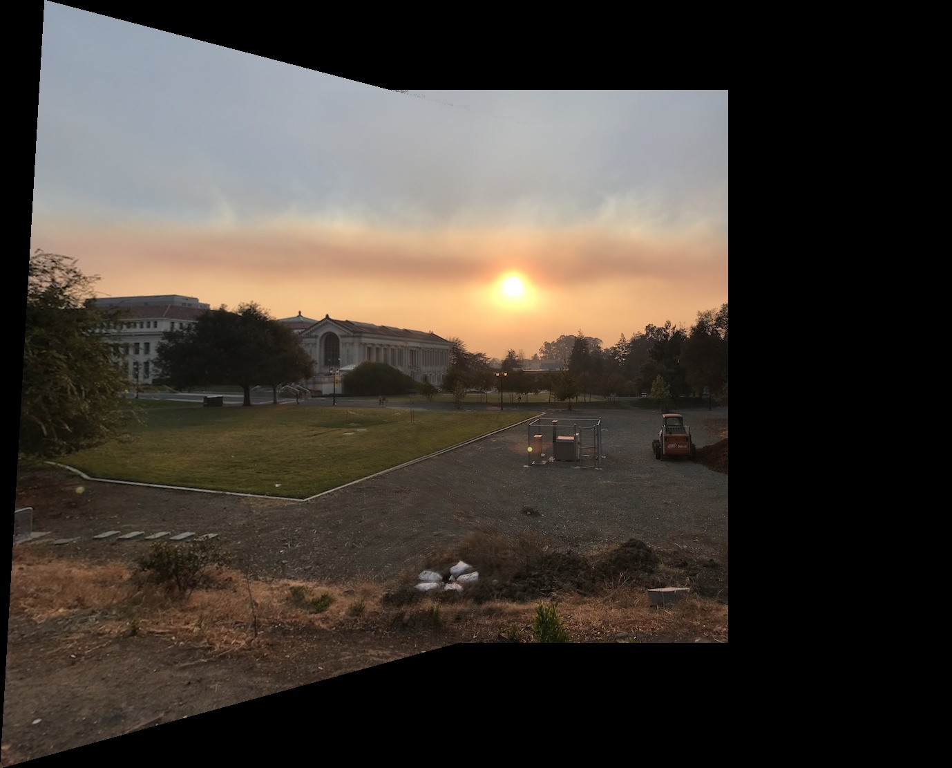
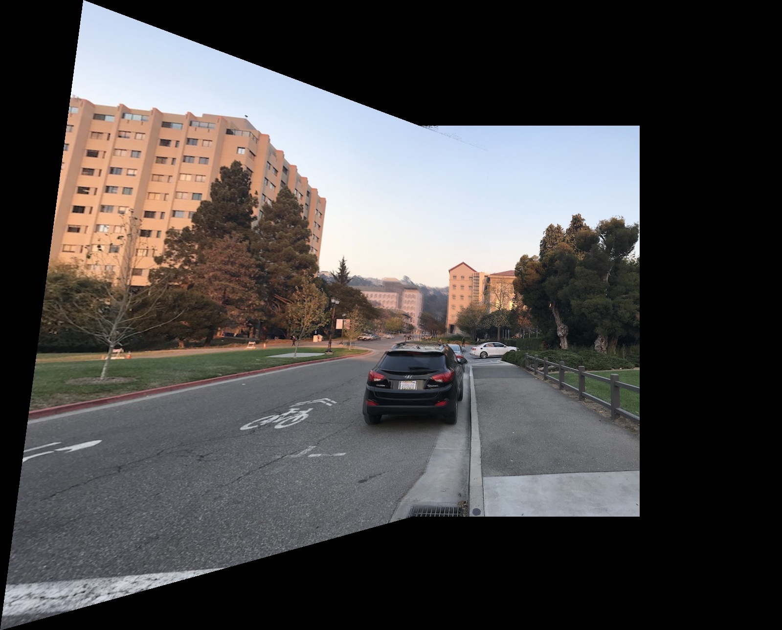
Mosaics
Manual Glade
Automatic Glade
Manual Car
Automatic Car
Manual Pug
Automatic Pug
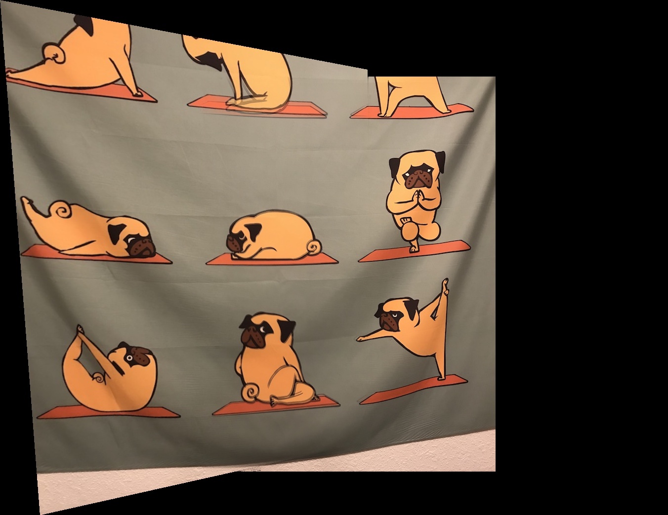
Between the automatic and the manual images, I don't think one of them is definitely better than the other. With the pug image, the auto seems to better align than the manual, but for the glade and car images, I'd say that it's difficult to tell which is which. I think this is a testament to my dedication in manually picking points by zooming in on the exact pixel.
What I've learned
There are many ways to take a set of corners and filter them down into correspondence points - ANMS, Feature Extraction, and RANSAC. One interesting part was filtering by the ratio 1-NN / 2-NN, as I would've merely chosen the 1-NN if I was developing this algorithm on my own. It was also really cool to be able to read a research paper and implement a majority of what it did, albeit with some shortcuts. I also learned to not confuse (x, y) coordinates with (y, x) coordinates, as that gave me a bug when I tried to apply the automatic feature points obtained in part B to my warping code from part A.