Project 6: Autostitching Mosaics

Credits to Mumu Lin for photos of San Francisco

Segment 1: Stitching Photos with Manual Correspondence

Part 1: Photo Collection

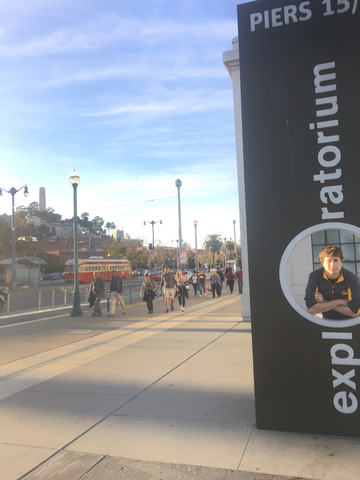
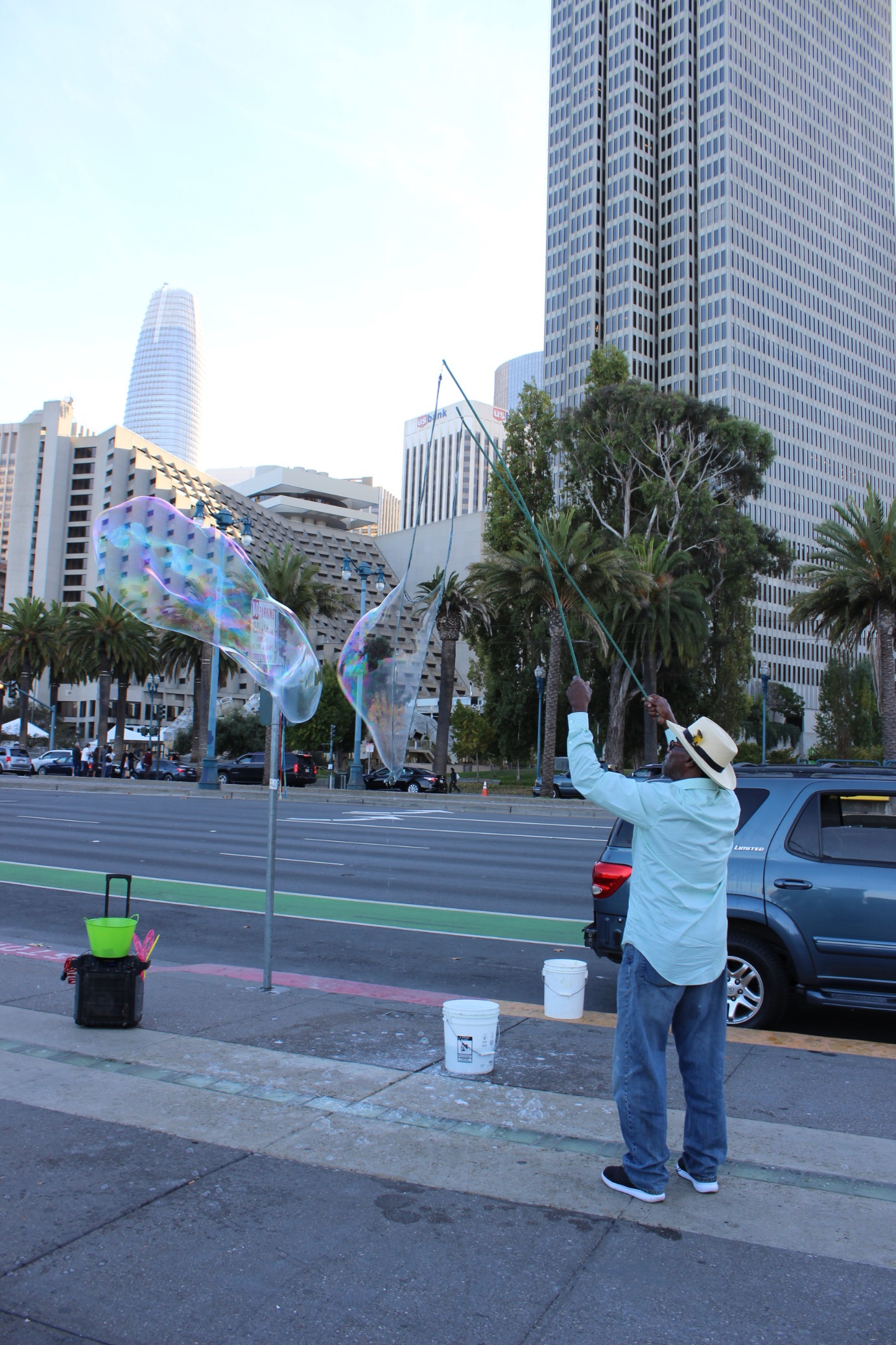
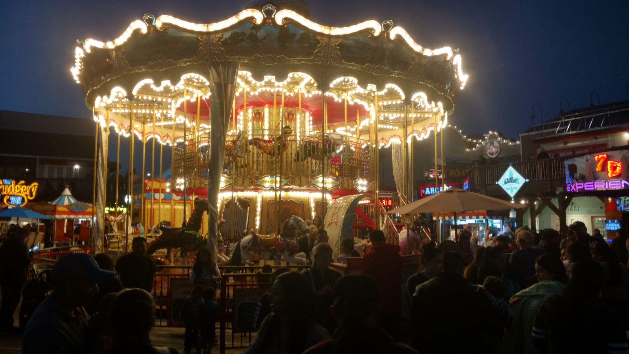
In order to obtain obtain some interesting photos for this stitching project, my friend Mumu and I took a day in San Francisco with a Canon EOS Rebel T3i camera. To take the photos, we stood at a fixed point, capturing images while rotating. The rotation was not as precise as could have been achieved with a tripod and some exposure settings were not locked, so some of the pictures came out slightly differently. However, I believe that we have obtained enough results to do some really interesting stuff.

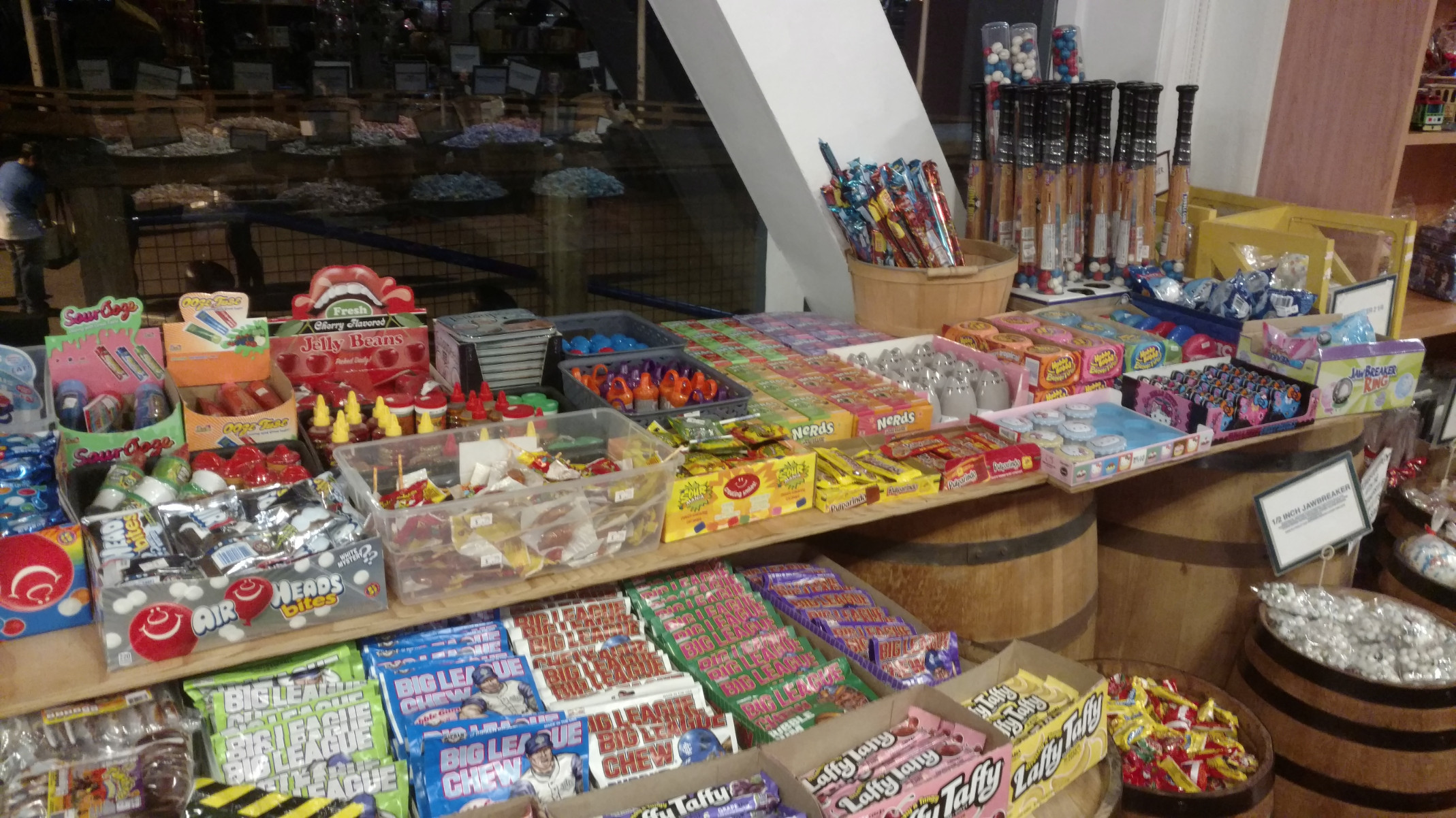
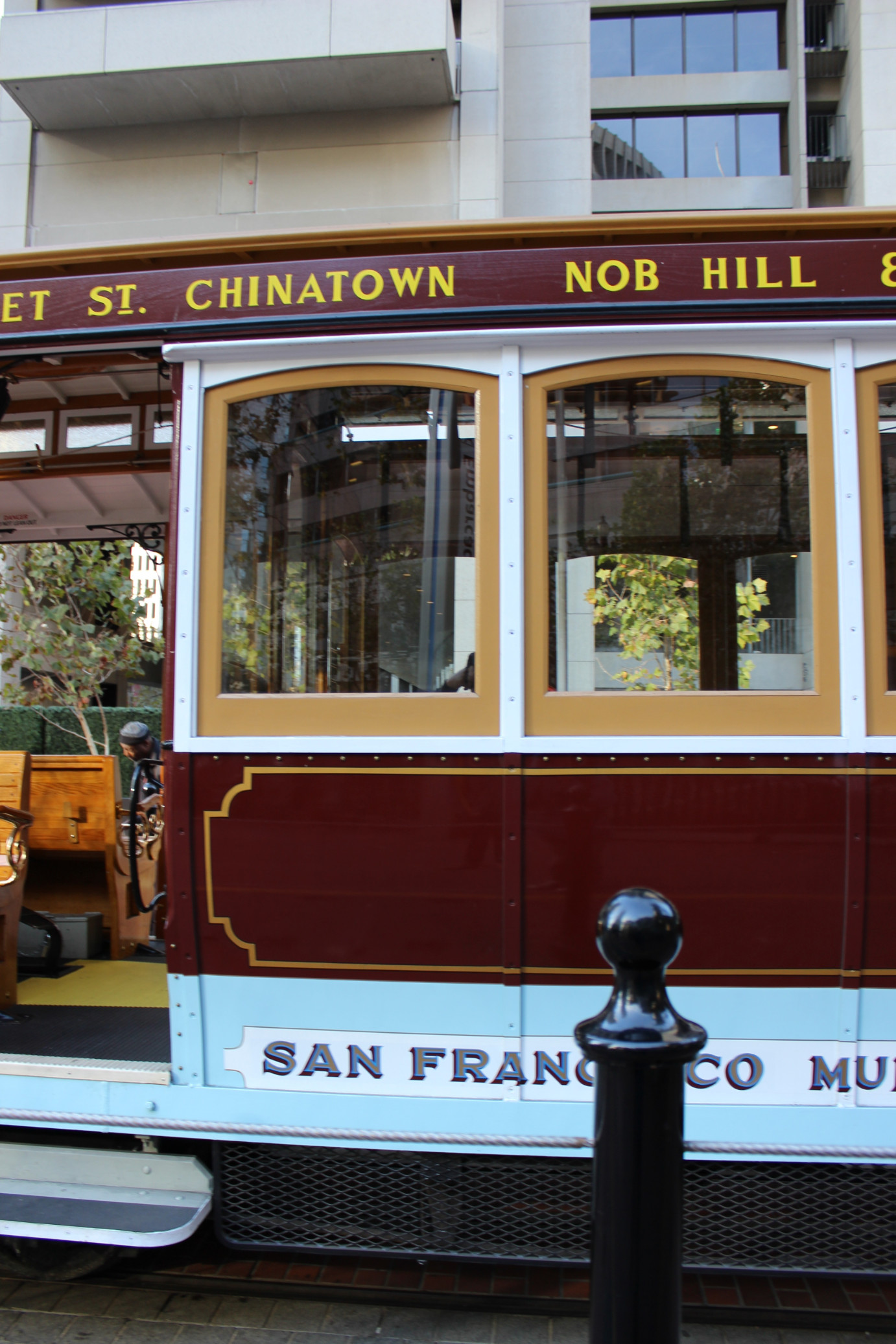
Here are some sample photos we obtained. Most of these are part of multiple sets of redundant photos:

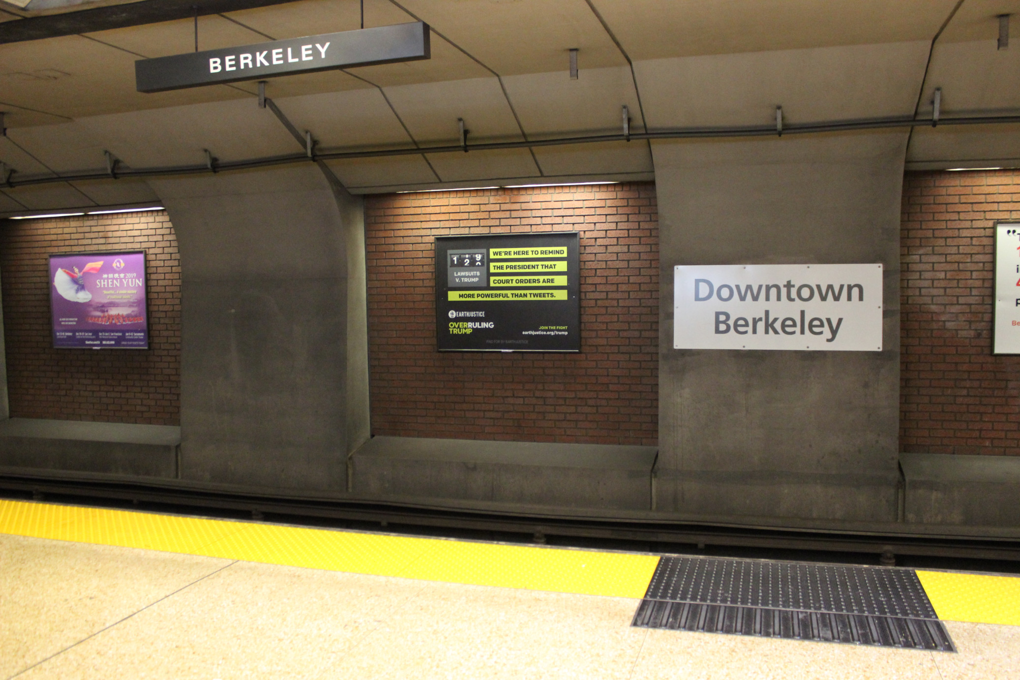
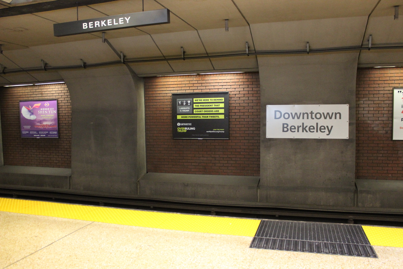
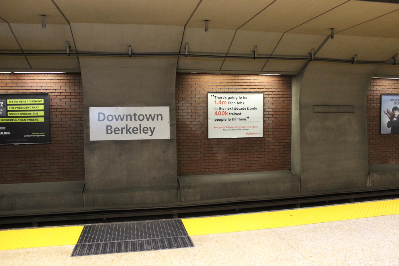
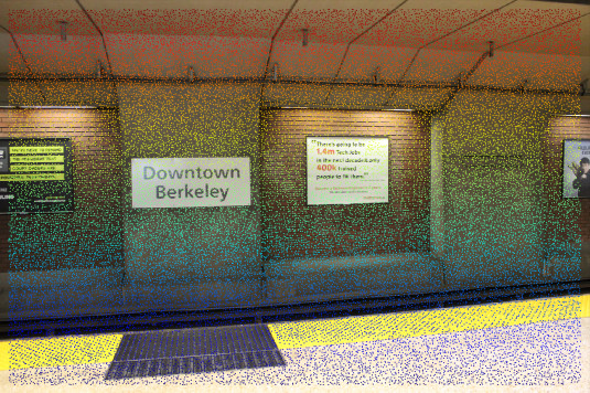
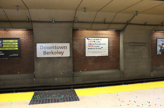
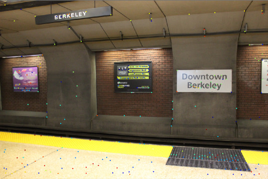
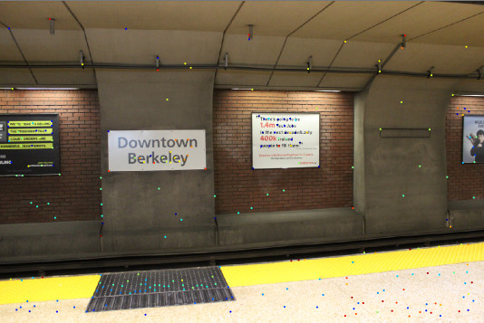
For simplicity, the two photos I will start working with are taken from Berkeley BART. I already defined 18 points of correspondence for making a mosaic out of them, which I will use at the end of this segment.

Part 2: Recovering the Homography

The goal here (similar to project 4) involves finding a 3x3 transform matrix used to translate pixels across the canvas. Such involves solving a system of linear equations to find a set of variables [h11, h12, h13, h21, h22, h23, h31, h32], with h33 constrained to 1.0 for normalization. That means that a correspondence needs at least 4 (x, y) points.

Each source point (x, y) will be used to create a row in matrix A along with the destination point...

[x1, y1, 1, 0, 0, 0, x1 * px1, y1 * px1]

[0, 0, 0, x1, y1, 1, x1 * py1, y1 * py1]

... with b being [px1, py1, ...].

Since some systems might be overdetermined (i.e. more than 4 points) I use numpy's least square solver for this task.

Part 3: Rectifying by Warping

Now that the homography matrix can be retrieved, we have to define a transform that applies to every pixel of the image. To apply a homography, dot product H * [x, y, 1] to receive w * px, w * py, w, the operation I will define as warp(x, y) -> px, py.

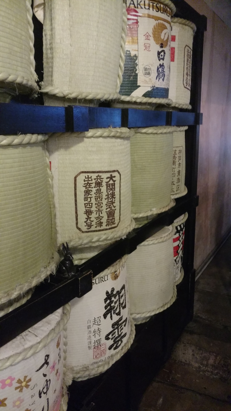
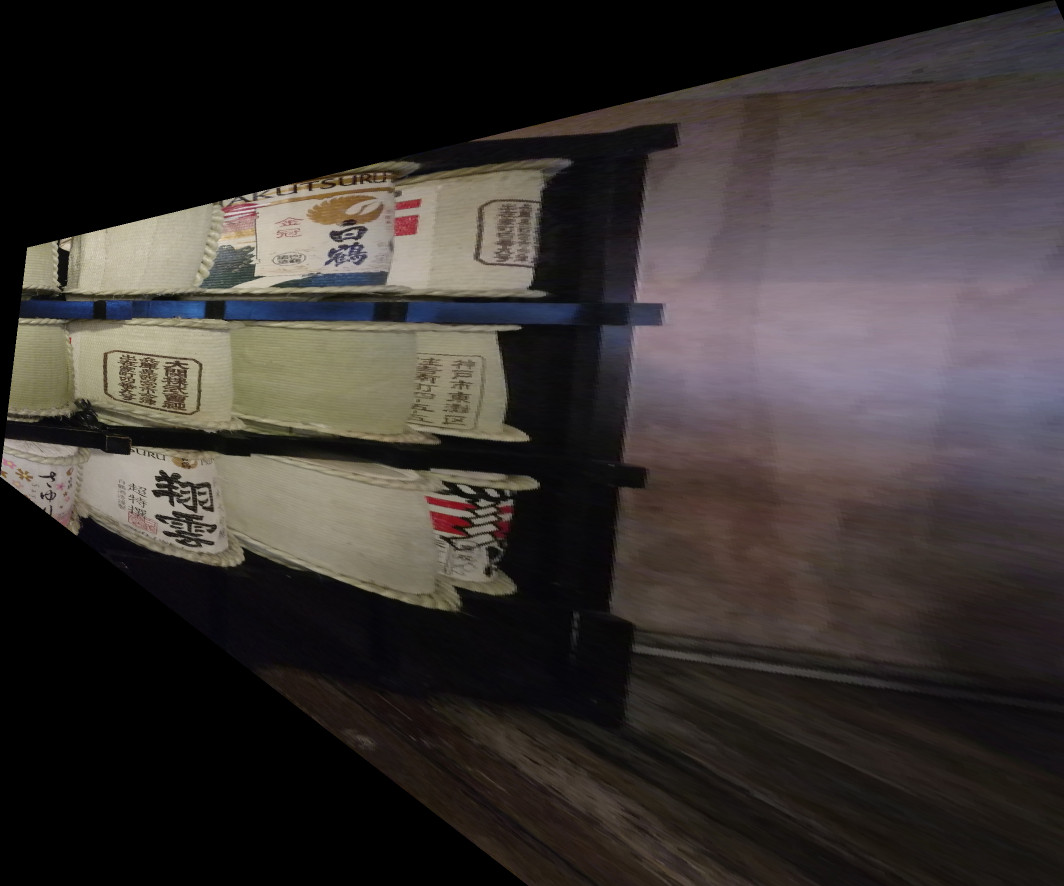
1. Find a bounding box to make the destination image by applying warp to the corners of the image.
2. Map pixels in the destination image to pixels in the source image using inverse warp (H^-1). Using forward warp to map source to destination might cause black empty space.

Here is the result on a secret door from a shabu shabu restaurant in Anaheim, warped to a square.

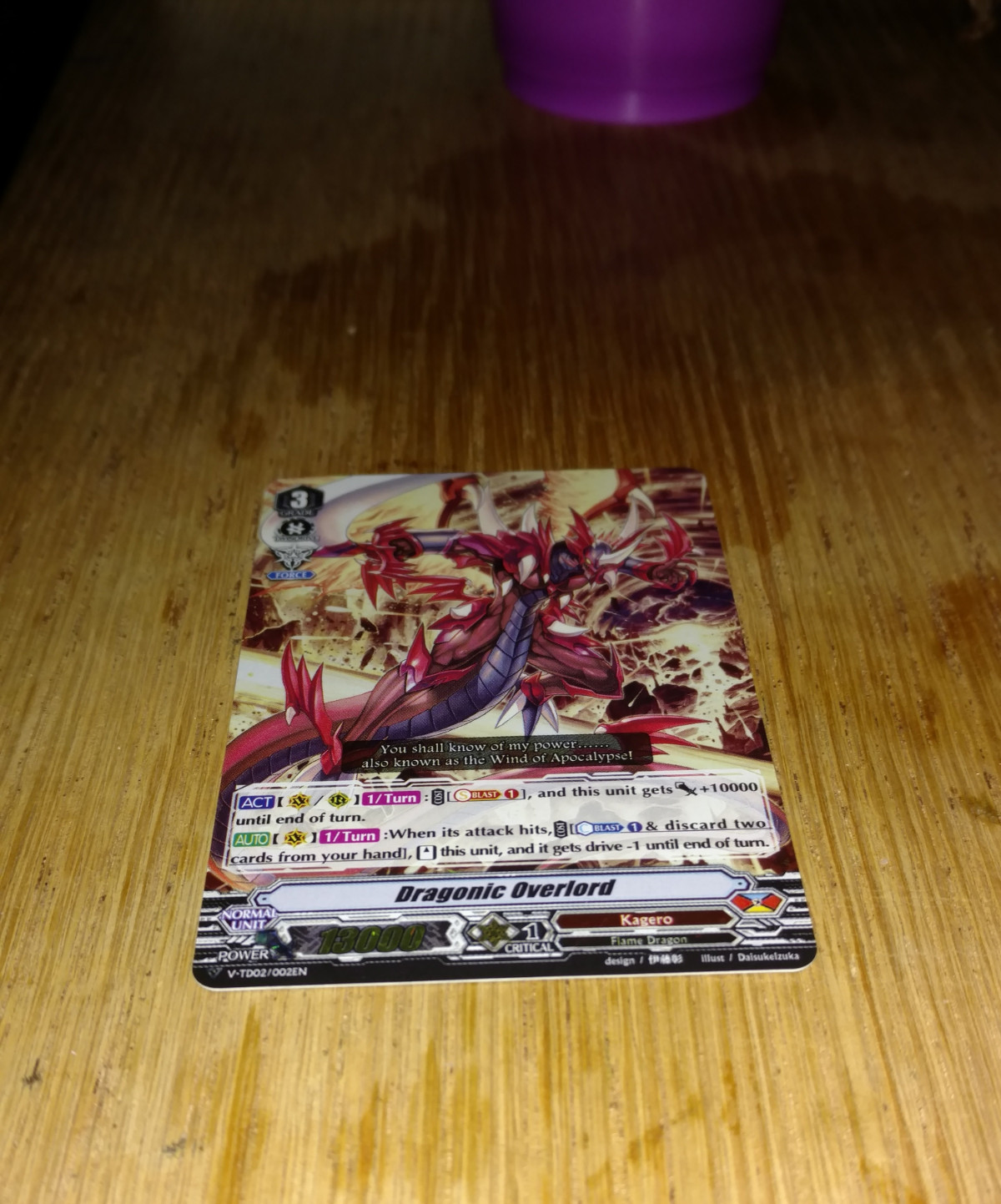
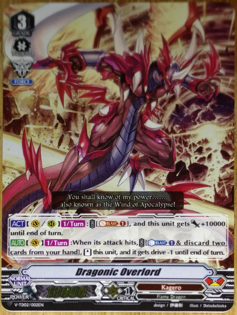
If you know the proportions of objects, you can also rectify into other shapes. For example, this Vanguard card has ratio 4:3.

Part 4: Photo Mosaics

This part is much the same as the previous, except the points will be overdetermined this time and we'll need to deal with blending multiple images.

Per some suggestions from other classmates, for intersecting portions of images, I used the max function to decide which pixel to use and it turned out pretty well.

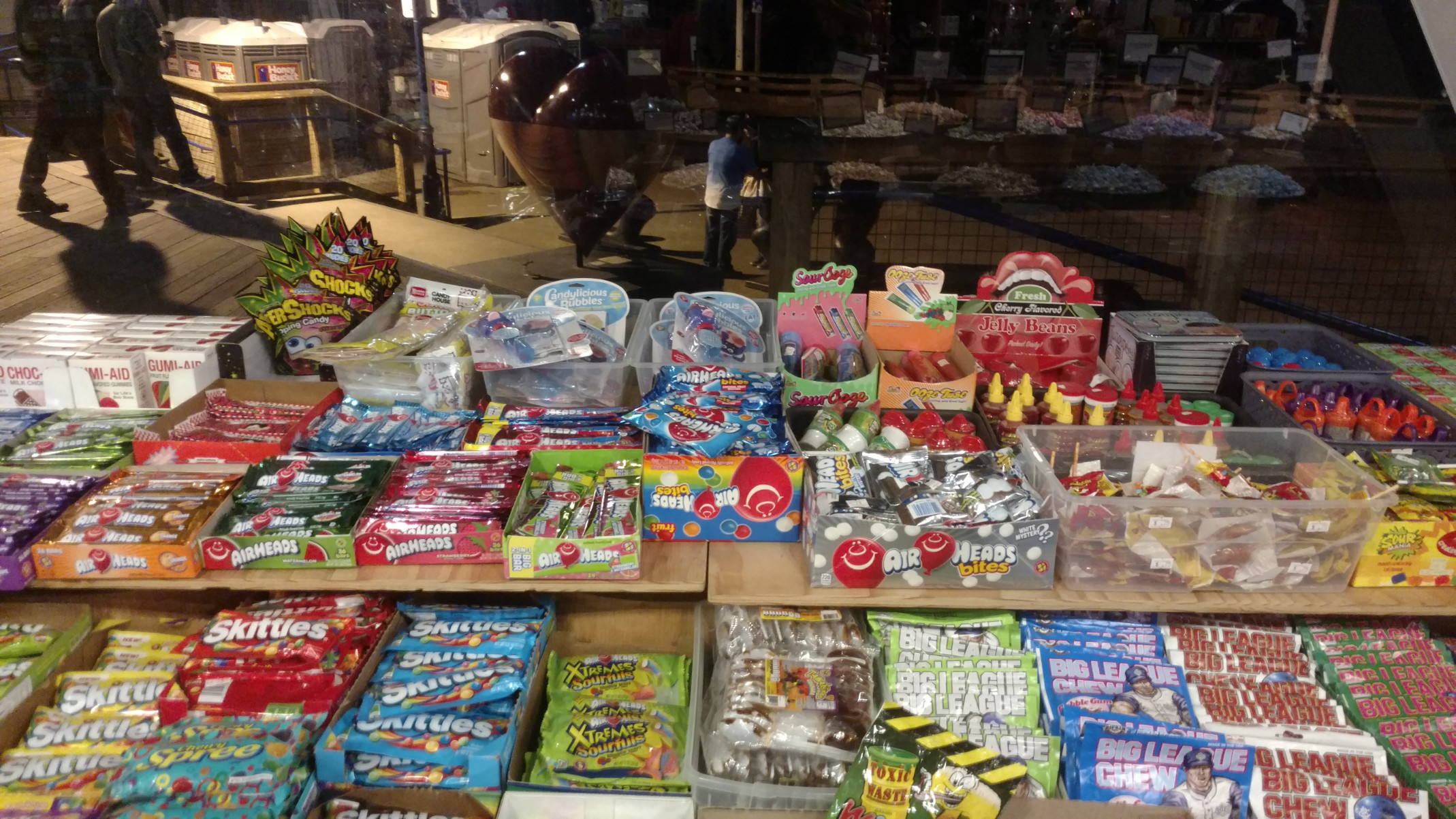
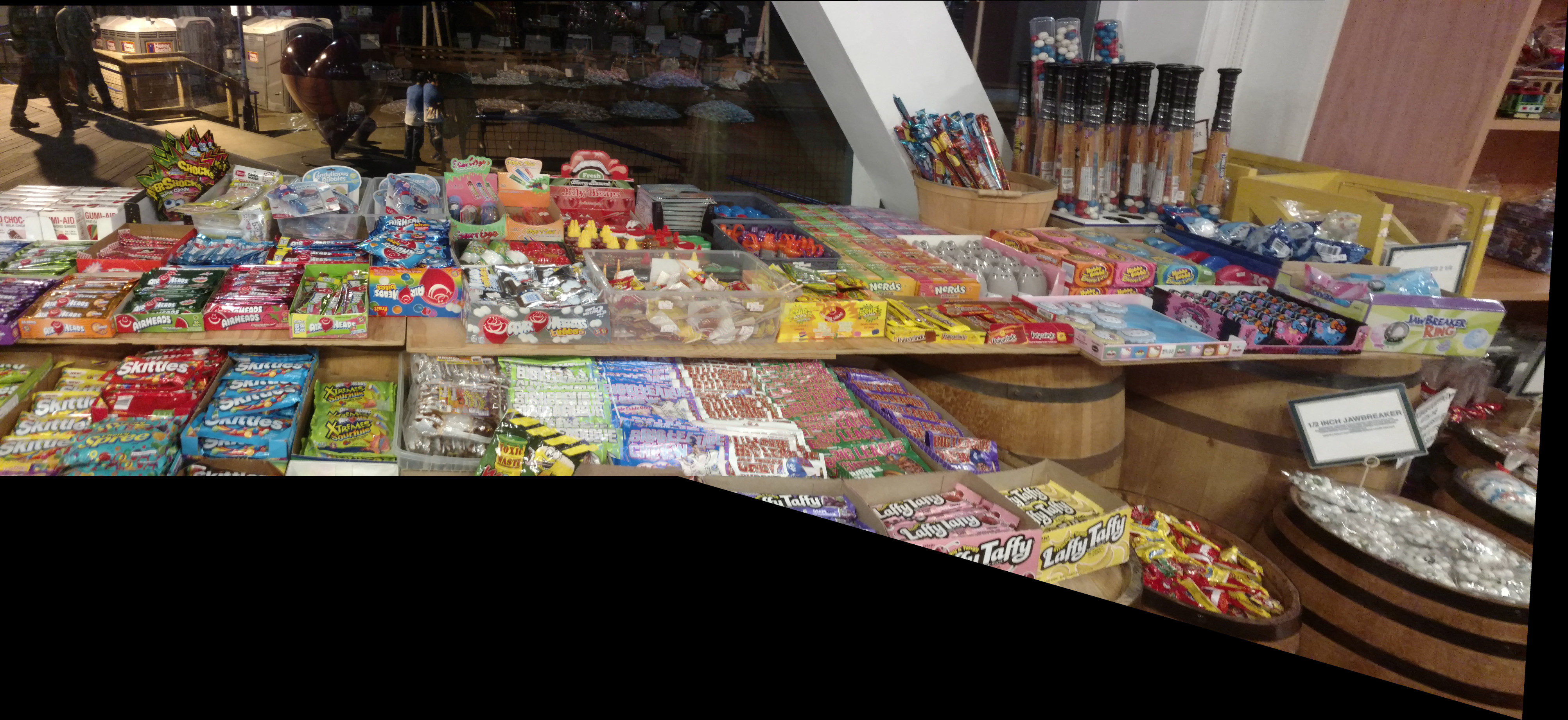
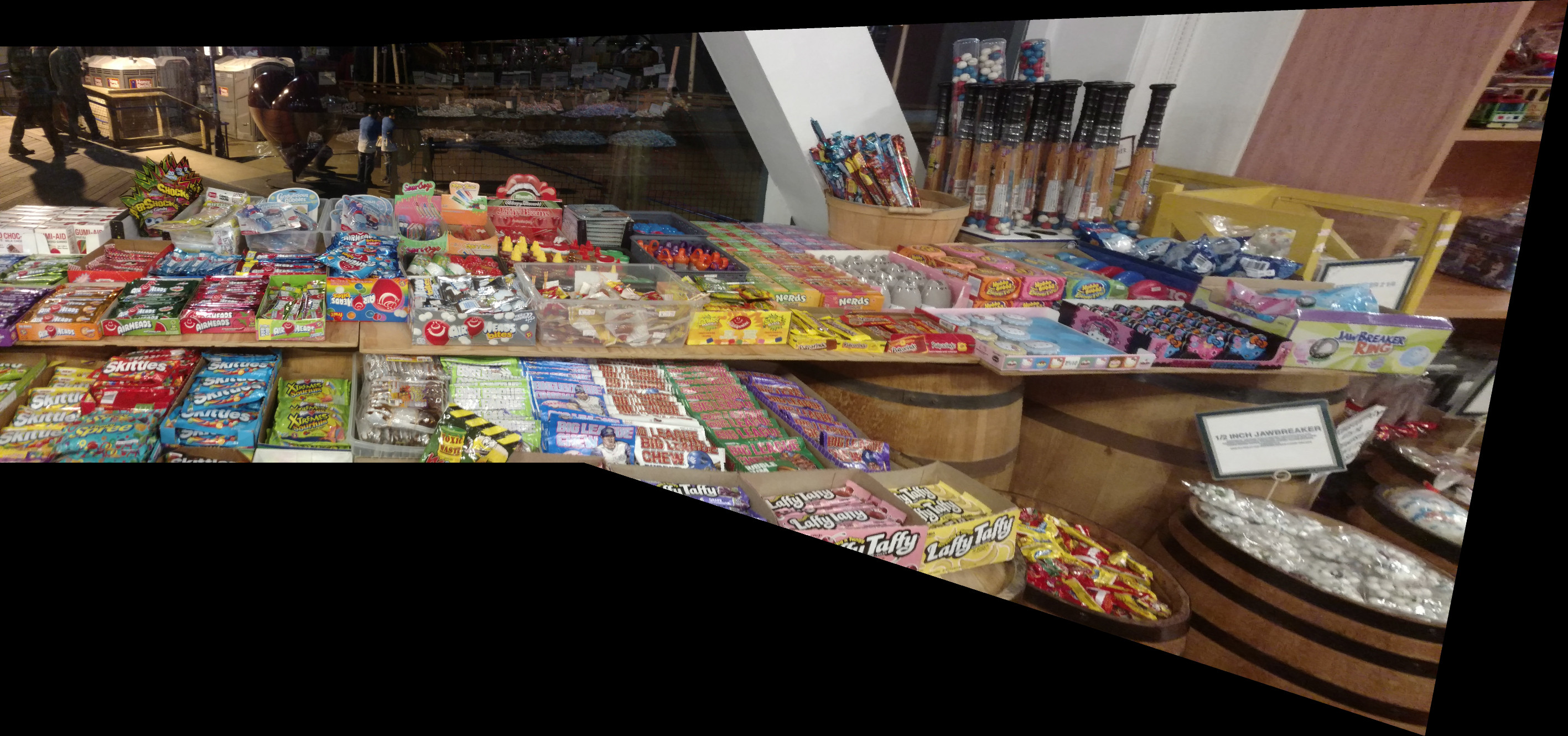
You'll notice the mosaic isn't quite perfect for the candy shop, due to the level of detail here. Better precision would require more correspondence points. Additionally, the guy in the background moved slightly, causing him to ruin part of the illusion. As you probably guessed, these mosaics are merely an approximation of the same scene, as there is a variable of time involved.

Again, defining correspondences that precisely transform the picture is hard:

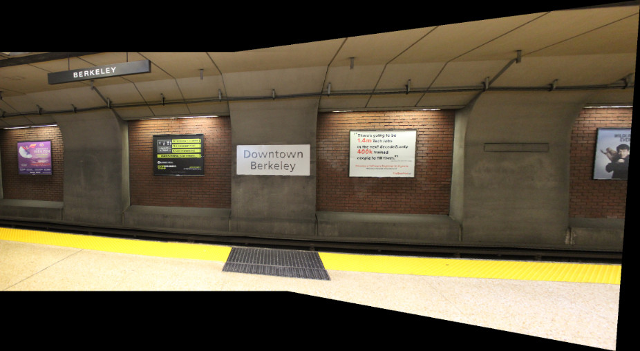
The BART one is probably the most convincing due to the simplicity of the geometry. In the next portion of this project, we'll see how to automatically (and hopefully better) define the correspondence points to make a mosaic.

Segment 2: Autostitching Photos with Feature Matching

Part 1: Harris Corners

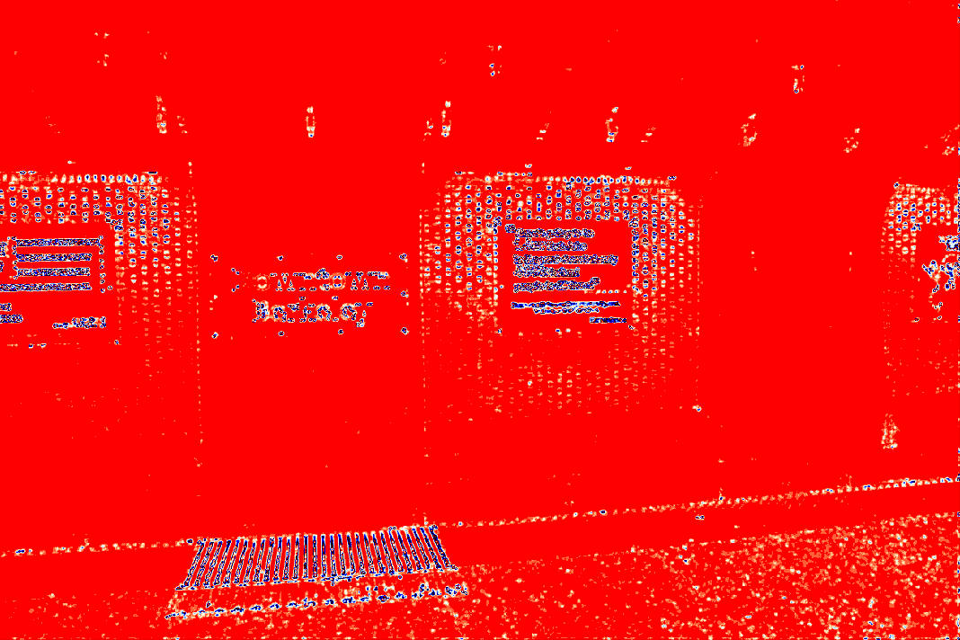
Given an input image, I, the idea is to generate a Harris matrix from a Gaussian image pyramid. Harris interest points are developed from the local maxima of a corner strength function. Most of this work is already done by a few provided functions in skimage. Below, I provided the results of running this function on one of my initial images.

The harris points alone are sufficient for calculating and matching features. However, in practice, the number of points is far too many to be computationally feasible. Adaptive Non-Maximal Suppression (ANMS) can reduce the number of interest points.

The algorithm involves starting an empty set for the final interest points (limited to, let's say, 250 points), choosing a suppression radius or in other words a minimum distance such that a point is a local maximum, and then decreasing the radius until enough interest points are found.

The goal of ANMS is to have an even distribution of points while also choosing the strongest corners -- otherwise we could just choose points at random. My implementation of ANMS, however, seems to favor strong points over even distribution:

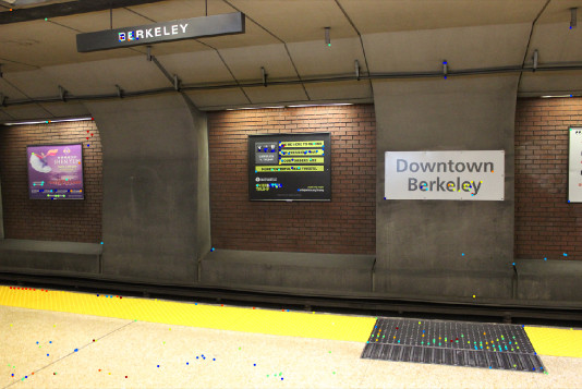
I solved the issue by increasing the min_distance of the points generated by the harris function, which not only improved the runtime of ANMS but also made the final result more accurate.

Part 2: Feature Description Extraction

Small 8x8 windows (features) can be sampled using 40x40 windows from points calculated by the previous part. After these are bias/gain normalized, they become reliable features for matching. Here are some of the features taken from each image:

Part 3: Feature Matching

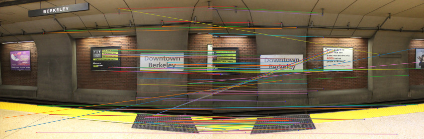
After extracting features from both images, the new goal is to find pairs of features that match well and thus can serve as good points for the homography matrix. Comparing each of the features to each other using the SSD function is sufficient to do the trick. Note the result on the images below. You may see features that locally look similar but as a whole are clearly not correct matches. The next part (RANSAC) will take care of this problem.

Part 4: RANSAC

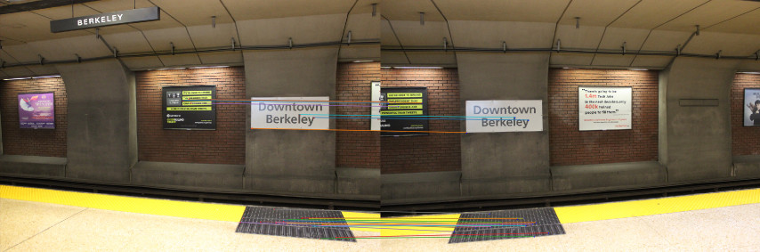
To remove outliers like many of the obvious ones seen in the above picture, I use random sample consensus. This relatively simple method runs for an arbitrary number of times (I do about a million). On each iteration, RANSAC chooses four random interest points, generates a transform matrix, and then checks how many feature matches line up with this homography matrix. The result is the largest set of agreeing interest points. Here is a RANSAC-filtered version of my matchings from above.

Now after all this careful work and choosing, I can compare whether the homography matrix generated by this overdetermined system warps the images as well as the manually chosen correspondences.

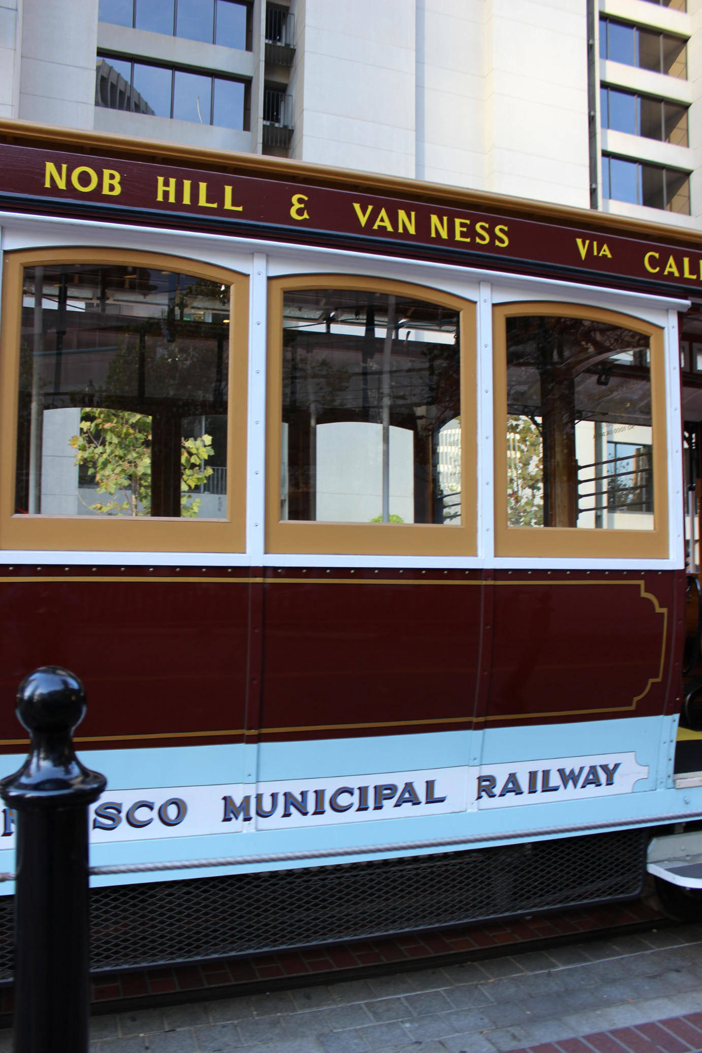
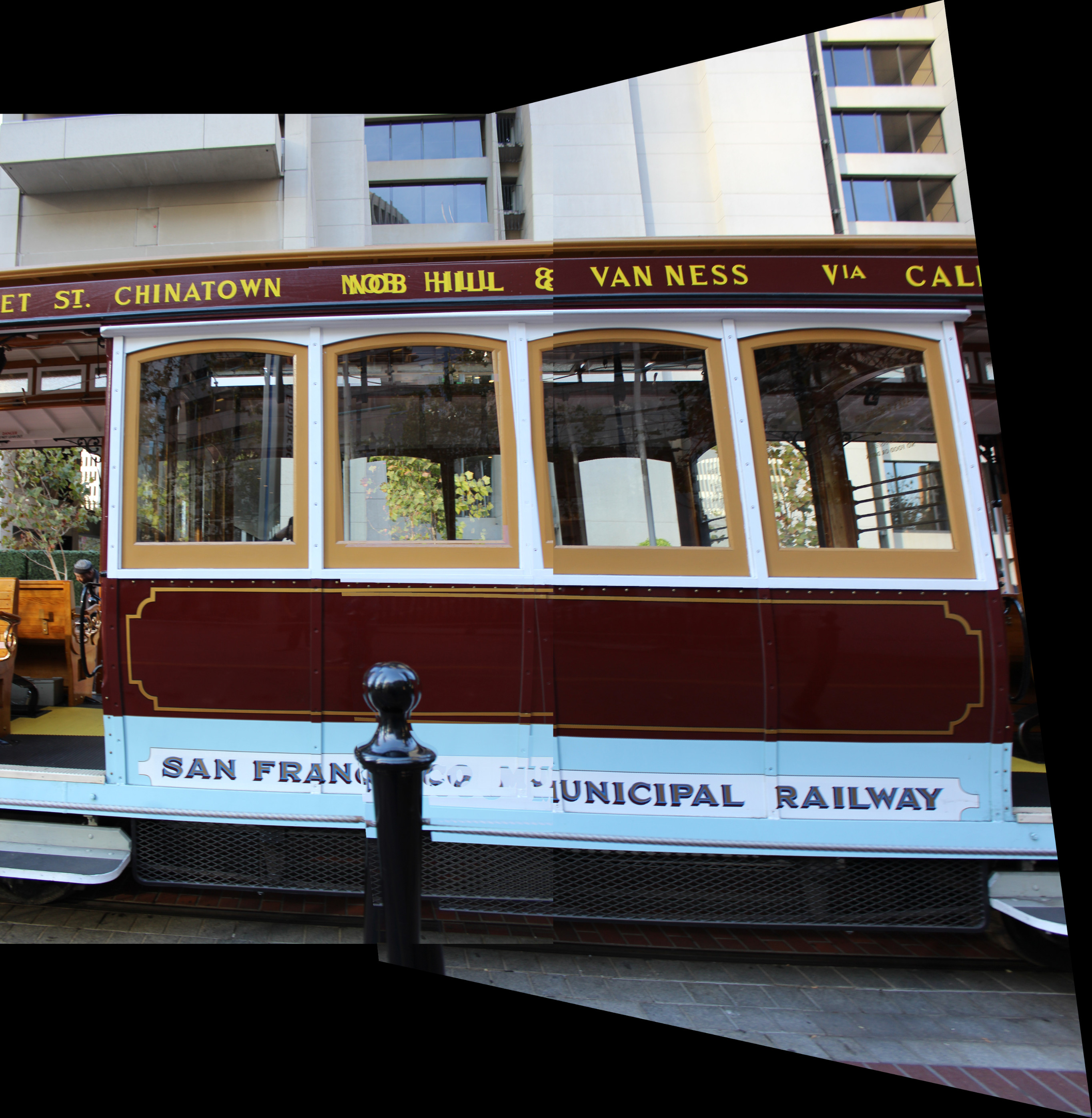
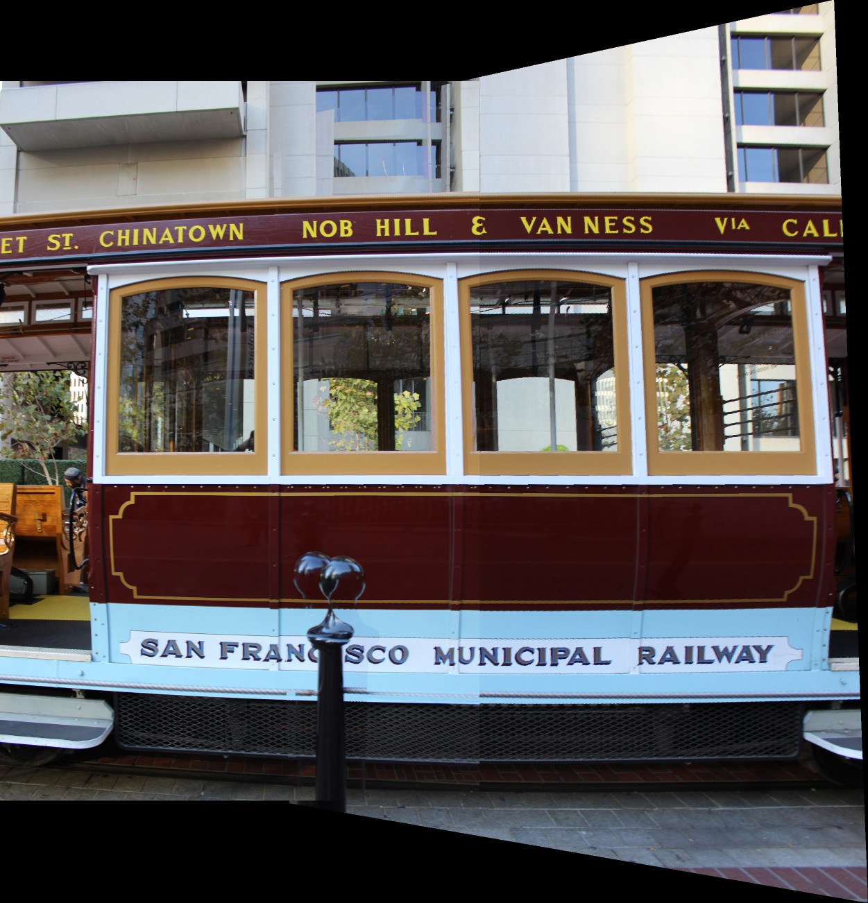
On moving to the cable picture, I noticed a couple things:

1. feature-matching was working properly but RANSAC wasn't finding enough points
2. RANSAC was simply too slow

In fact, RANSAC's inability to match points reveals not that RANSAC is the problem, but that the pictures Mumu and I took weren't perfect. The pole in front of the cable car actually was now in a different position due to slight camera translation in the physical world. My solution was to make RANSAC a little more forgiving, and it works well now (sometimes).

1. don't check random correspondences that have been seen before (it's redundant)
2. increase the error tolerance to about 5 pixels -- mismatched points are often wildly mismatched

I got a pretty good output after doing this:

Another note -- this automatic implementation doesn't seem to work as well on large images. Now, as a test of strength, another go on the candy shop:

Conclusion

Seems that auto-stitching proves to be less time intensive and more accurate than manually defining points -- however, it is more prone to huge mistakes than a human correspondence maker (i.e. sensitivity to scale, rotation, and image size). If I wanted to and had more time, I would make the automatic stitching invariant to rotation / optimize further, but I think it's okay to cut it off here for now. It was a fun exploration into practical use of transforms to make panoramas.