We solved for a homography in order to change the perspective of an image. Using our homography, we rectified images (warped a planar object to the
foreground plane). Then, we created an image mosaic. I took my pictures using my iphone and the burst camera mode.
We need 4 points to define a homography. Recall that a homography is defined by
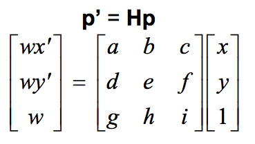
where p' is the desired coordinates and p is the coordinates of the original image. By multiplying Hp out and substituting for w, we can create a system of linear equations that allow us to solve for the unknown values of H by using least squares. We can simply H by letting i=1 since w is just a constant. We add an extra equation to force i to equal 1.
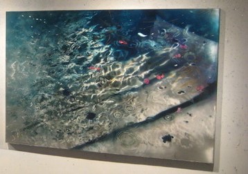
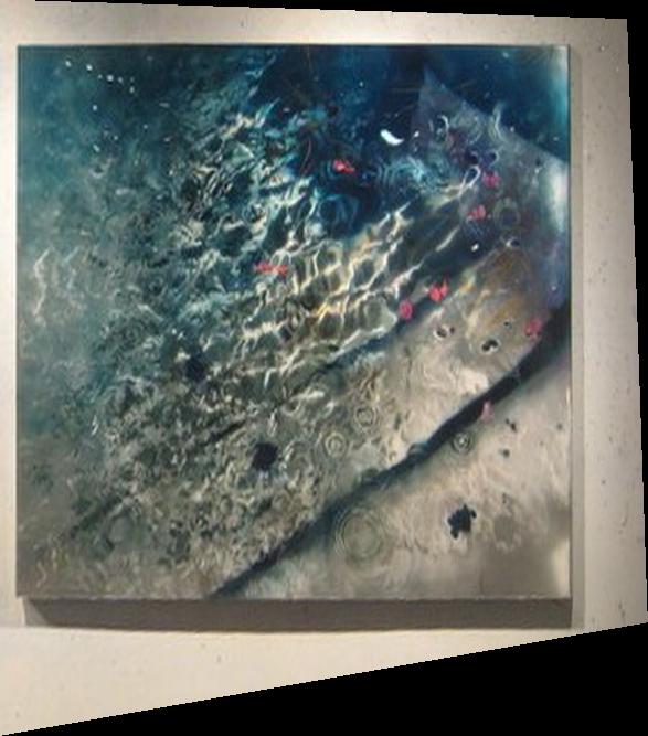
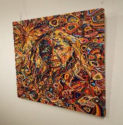
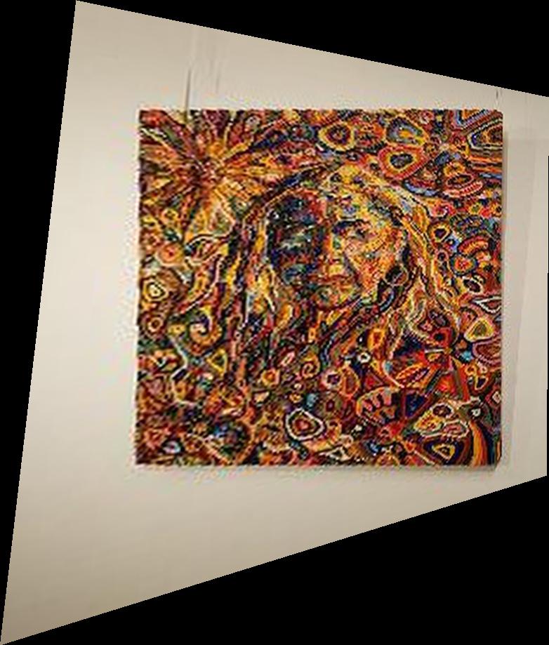
To rectify an image, we need to define four points on a planar object in the image that we wish to warp to the foreground plane. Using those 4 chosen points and the predefined coordinates of a square, I computed a homography mapping the image to the foreground plane. Then, I warped the image to the foreground to complete the rectifying process. To warp the image, I first calculated a mask of the resulting image by
applying the homography to the four corner points of the original image. Then for every pixel in the mask, I applied the inverse homography to find the coordinates of the desired pixel value in the original image. Since those coordinates may not be integer valued, I interpolated the image using
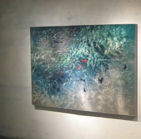
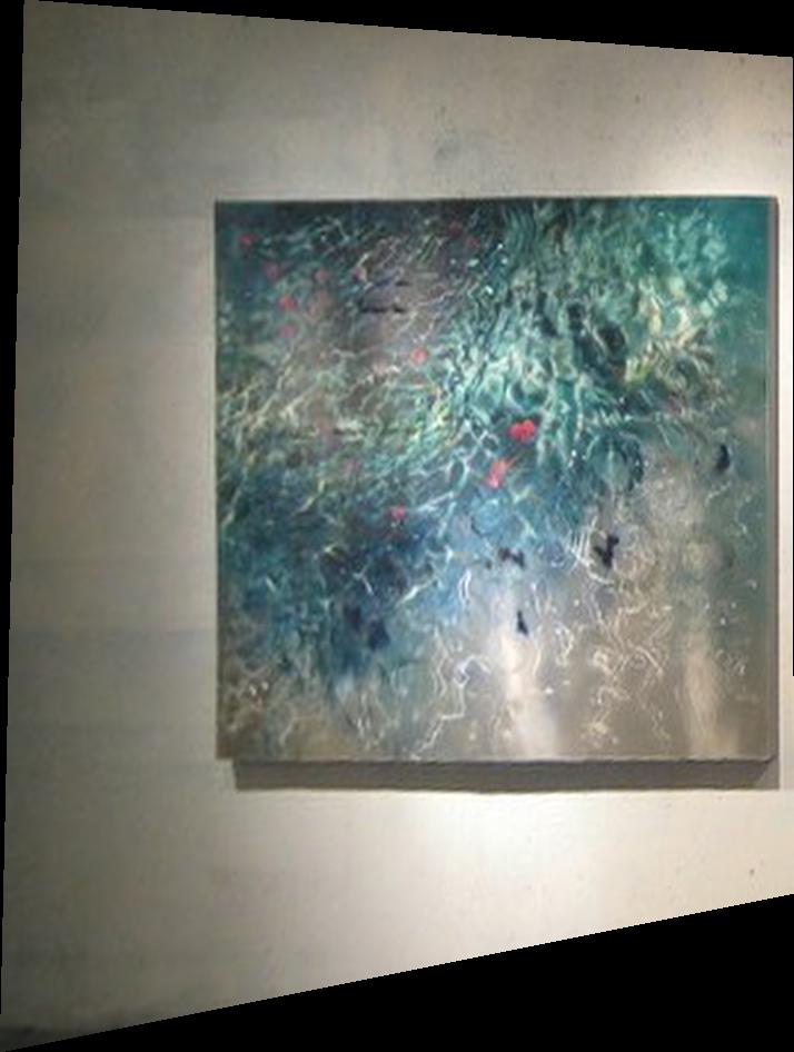
scipy.interpolate.interp2d. I rectified various artworks that were taken from an angle to get a frontal view of the piece.
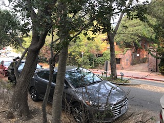
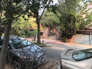
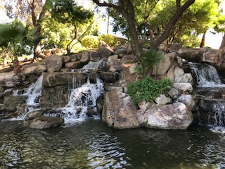
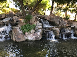
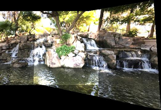
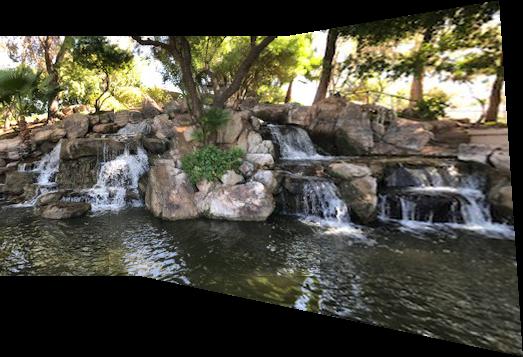
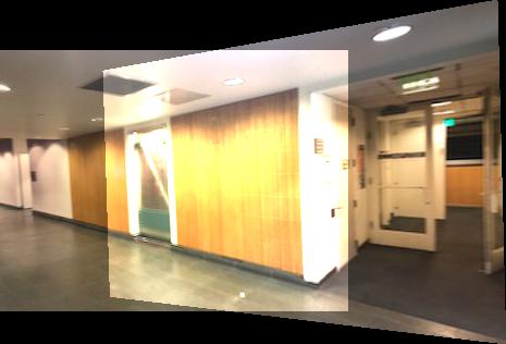
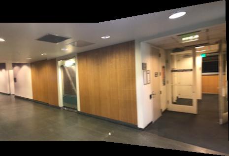
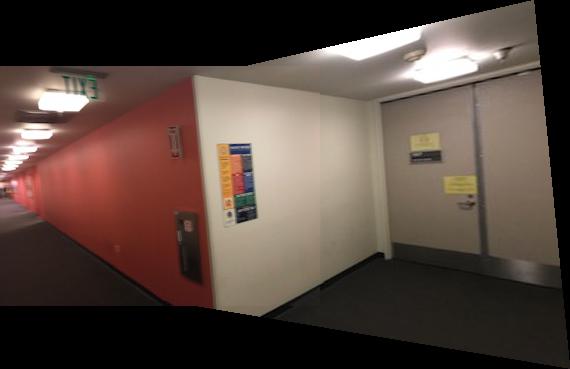
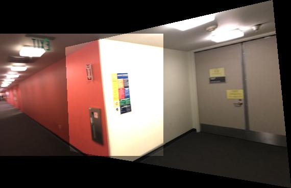
Finally, I created image mosaices by combining two source images into one coherent mosaic. To create the mosaic, I first defined at least 4 coorespondace points between the source images. I then used the coorespondances to compute the homography that warps the right source image onto the left source image's plane. Using that homography, I warped the right source image and then combined it with the left source image. I blended them by taking the maximum value of the two images. I experimented with different number of coorespondances and saw I could typically get decent results with 8 - 12 pts. More points did not tend to help and were hard to identify. The unblended results were obtained by naively adding the left image and the warped right image together.
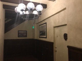
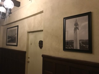
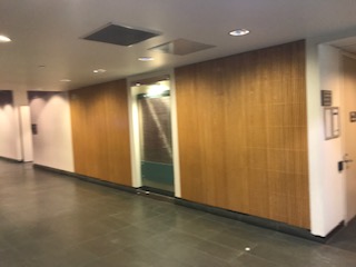
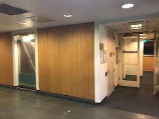
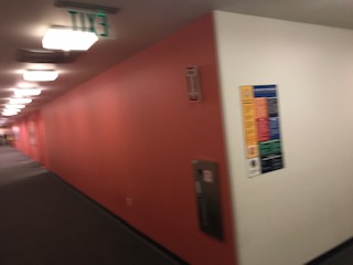
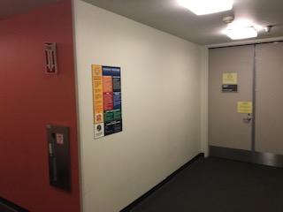
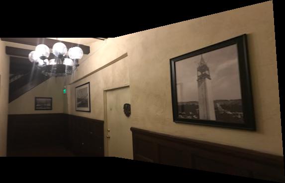
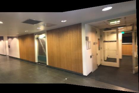
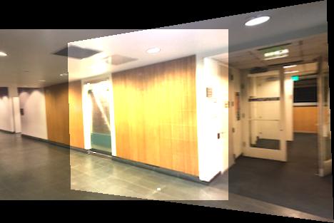
I tried making moasaics around corners in Soda. These images were challenging to identify features on since they were mostly walls.
What I learned
Homographies are powerful!
I saw how a homography can be used to change an image perspective and recover a distorted image.
Homographies also allow us to stitch together multiple images taken from different rotations together
into a coherent mosaic.
I learned defining the coorrespondance points was challenging and should not be done by a human hand. Humans are too prone to
error. The coorrespondance points must be evenly distributed across the overlap between the two images. The points must be in both foreground and background of the image, and they cannot skewed towards one side of the image. If the image data is nice, then I could get decent results with fewer points. Unfortunately, no amount of coorrespondances makes up for blurry images with too little overlap and lighting changes.
Part 2
Overview
We use automatic corner detection to stitch mosaics together without a human mapping correspondances. We used Harris Corner Detector to find corners in the image.
Adaptive Non-Maximal Suppression
To make sure our corners were spread evenly across our image, we used Adaptive Non-Maximal Suppression algorithm.
In the algorithm, we iterate through each Harris Corner and calculate the point's suppression radius as the distance to the closest point that is 90% stronger than the current point.
Recall that the strength of a corner is defined by
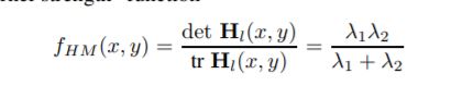
which is the deteriment of the gradient matrix over the trace of the gradient matrix.
Explictly, a point's minimum suppression radius is defined by

where f is the corner strength and gamma is the set of all points. I kept only points whose suppression radius was greater than 12. In order to allow feature descriptors to have a 40x40 window, I only kept points that were 20 pixels or more away from the edge.
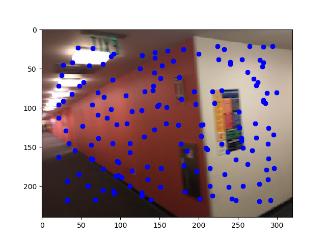
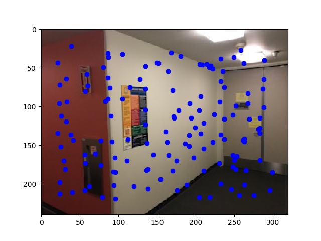
Below are some examples of Harris Detection Corners using ANMS.
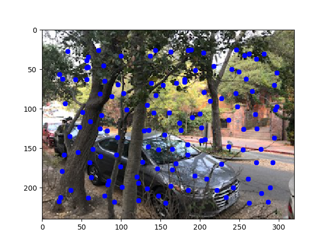
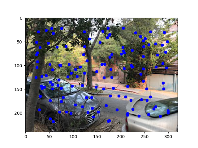
Feature Descriptor
Each Harris Corner must have a feature descriptor that allows us to find similar points in the images and create a correspondance. I created an 8x8 feature descriptor by downsampling the 40x40 pixel patch centered on the the Harris Corner. After I create the 8x8 patch, I flattened it into a vector to be easier to work with and normalized the vector to have 0 mean and unit variance. The bias/gain normalization is important to make our feature descriptors invariant to affine transformations.
Feature Matching
For every point in the first image, I found the two nearest neighbors in the feature descriptor space. As a similarity measure, I used the Euclidean distace (aka L2 norm) in the feature space since my feature descriptors were converted to be vectors. I used the Lowe thresholding to decide if a two points formed a good coorrespondance. Specifically, I defined a good coorrespondace to be a point in the first image such that the ratio of its first nearest neighbor in the second image over its second nearest neighbor in the second image is less than 0.5. The intuition is that the first nearest neighbor is much more similar to the point in the first image than the second nearest neighbor. If the two nearest neighbors are too similar, then there are multiple equally good mappings from the first image to the second.
A good coorespondance should have only one possible mapping from the first image to the second, not multiple mappings.
Below are examples of the coorrespondance between two images.
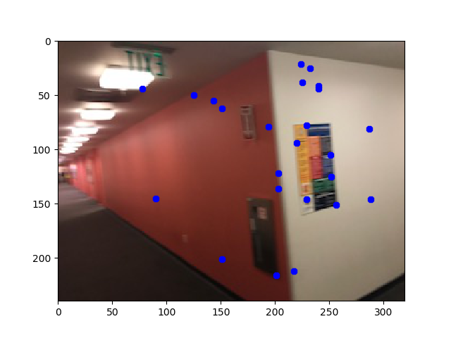
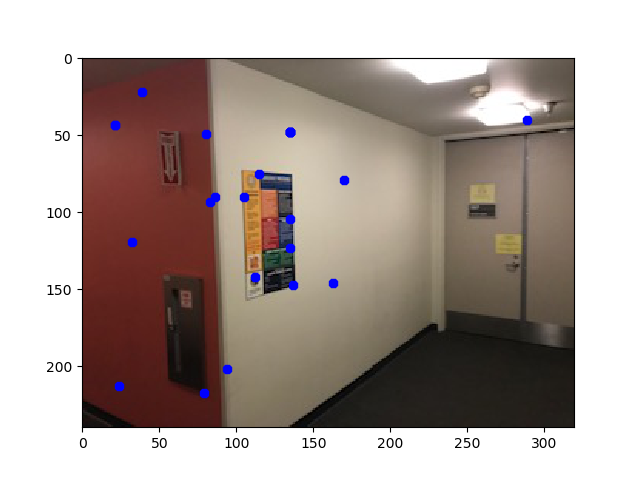
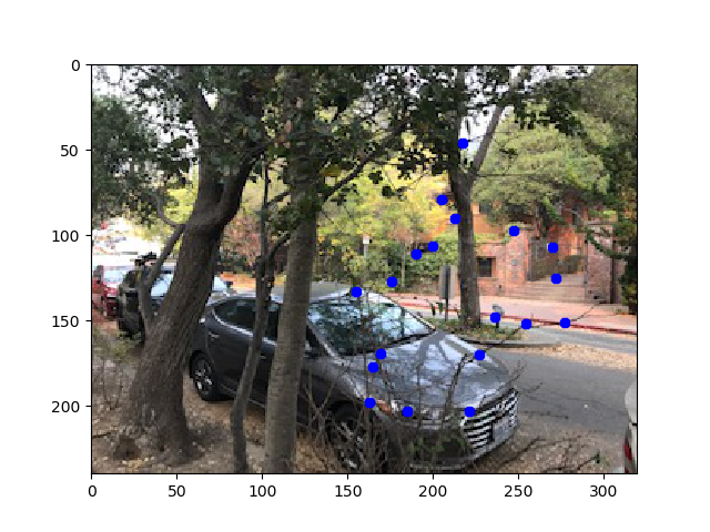
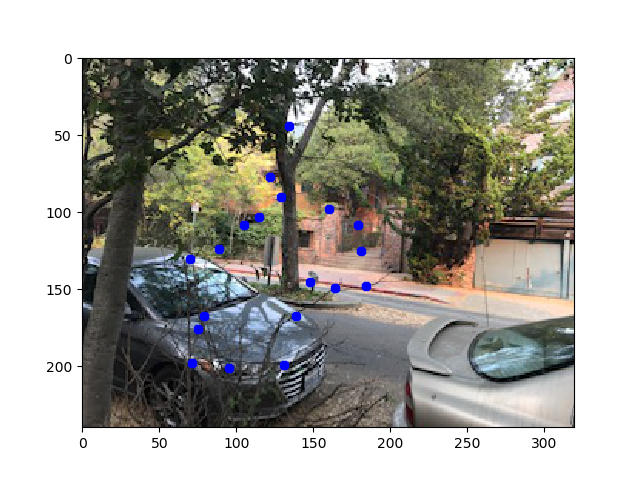
Note some of these coorrespondances are not the best and would not be chosen by a human. We fix this in the next section.
RANSAC
To make the code more robust to outliers in our coorrespondances, we used RANSAC. In RANSAC, we randomly select a subset of 4 coorrespondances and compute a homography. We then apply that homography to the points in the first image and see if we get the coorresponding point in the second image. We count the number of inliners or where our calculated point is the same as the point in the second image. I tried 300 homographies and picked the largest inliner group as the best homography. We used the largest inliner group to compute the homography that was used for the stitching.
Results
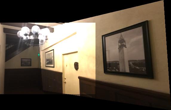
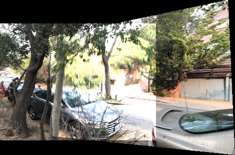
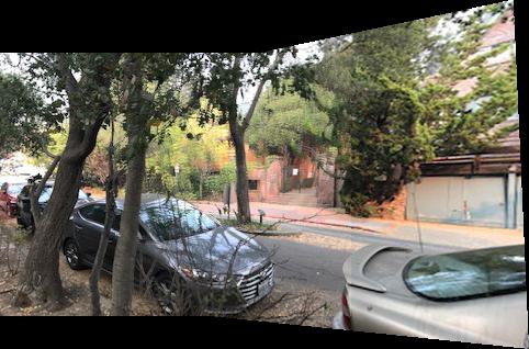
Automatic Blended
Largest Inliner group was 55/144
Automatic Unblended
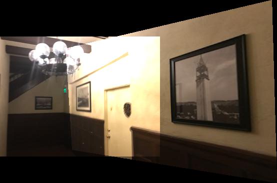
Images Combined
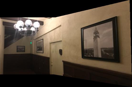
Blended Mosaic using 12 Coorrespondances
Automatic Blended
Largest Inliner group was 103/216
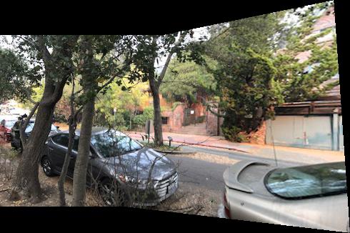
Automatic Unblended
Images Combined
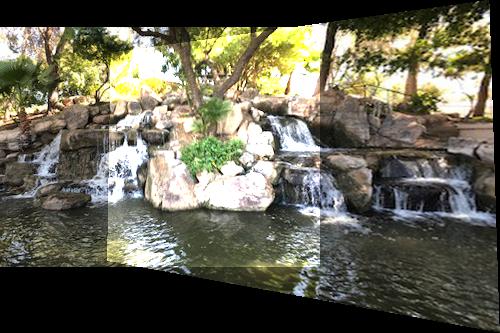
Blended Mosaic using 12 Coorrespondances
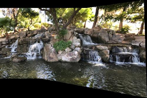
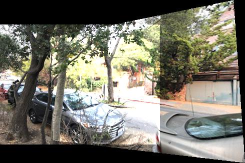
Automatic Blended
Largest Inliner group was 156/144
Automatic Unblended
Images Combined
Blended Mosaic using 8 Coorrespondances
Automatic Blended
Largest Inliner group was 111/219
Automatic Unblended
Images Combined
Blended Mosaic using 20 Coorrespondances
Automatic Blended
Largest Inliner group was 27/103
Automatic Unblended
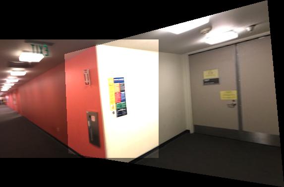
Images Combined
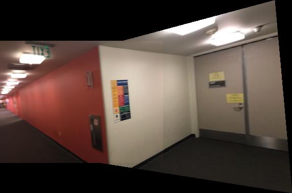
Blended Mosaic using 16 Coorrespondances
What I learned
I learned how to use Harris Corner Detection, ANMS and RANSAC to create automatic mosaic stitching. I think the results of automatic stitching were comparable to the results found by human choosen coorespondance. However, the automatic stitching was much easier to use as I didn't need to define coorrespondances and then refine them by hand to improve the mosaic. The automatic stitching struggled on the same images I struggled to do by hand (eg the soda corner with bad lighting).