Overview
In this project, we use various methods to warp images and create photomosaics (like panoramas).
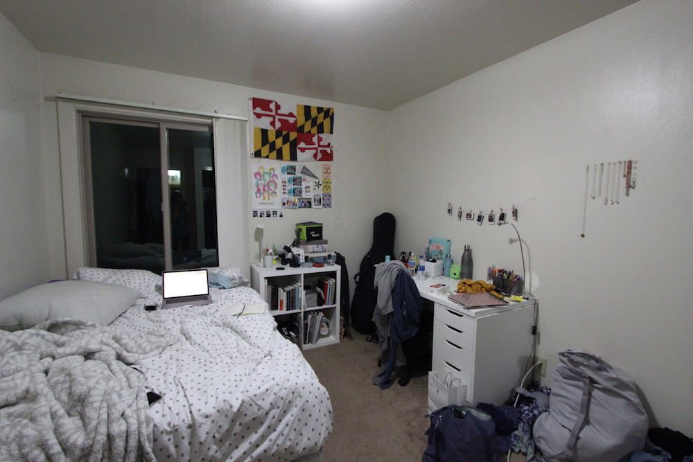
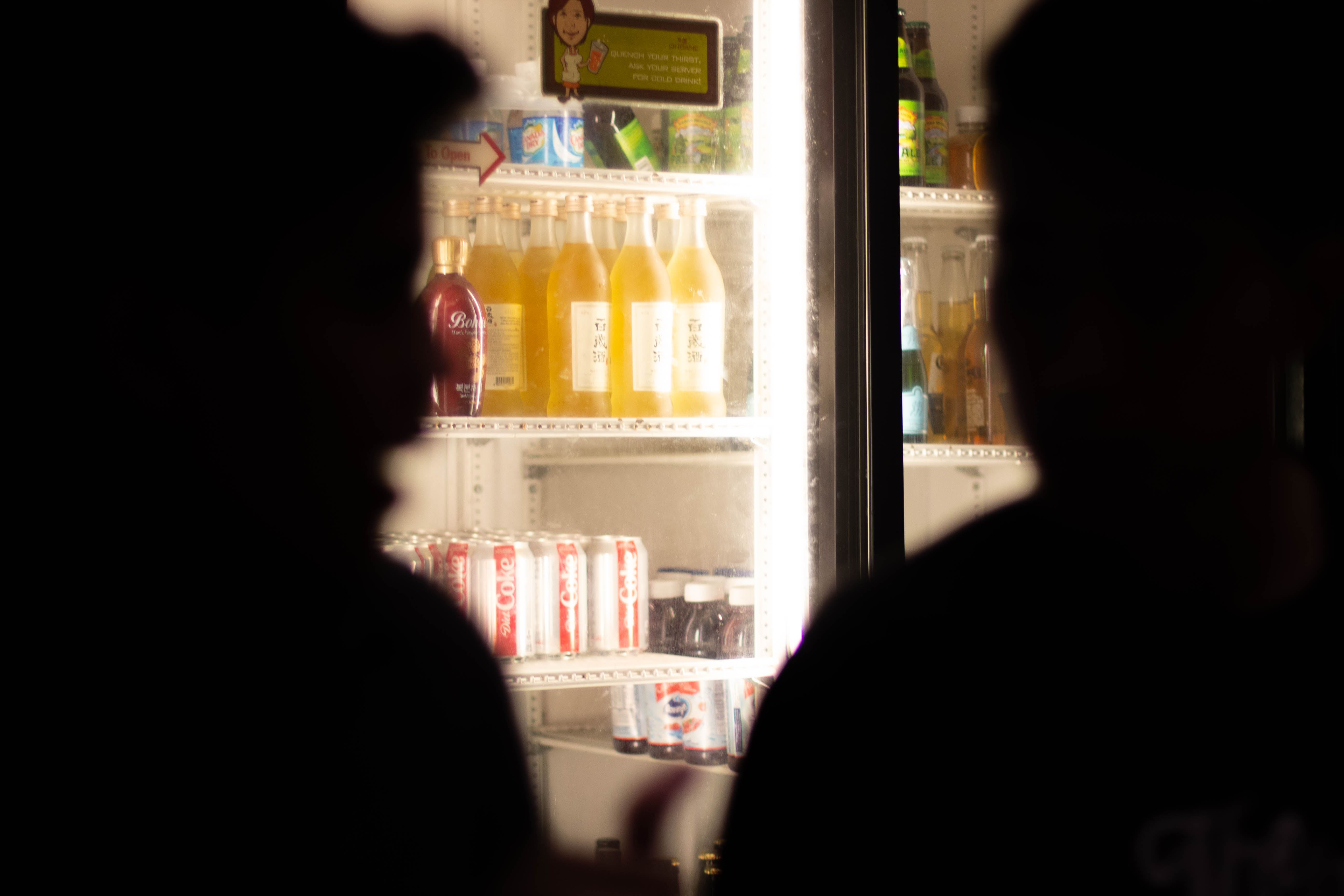
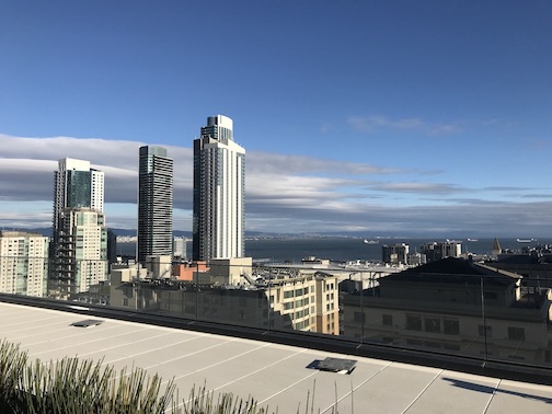
Part A1: Shoot and Digitize Pictures
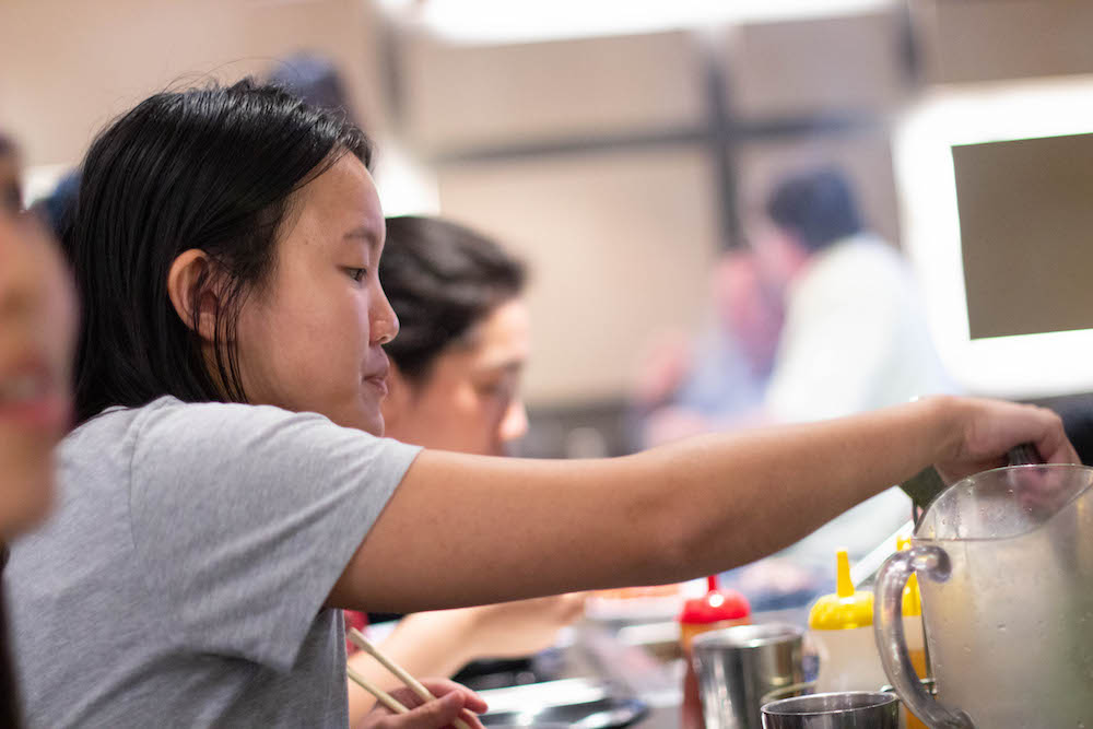
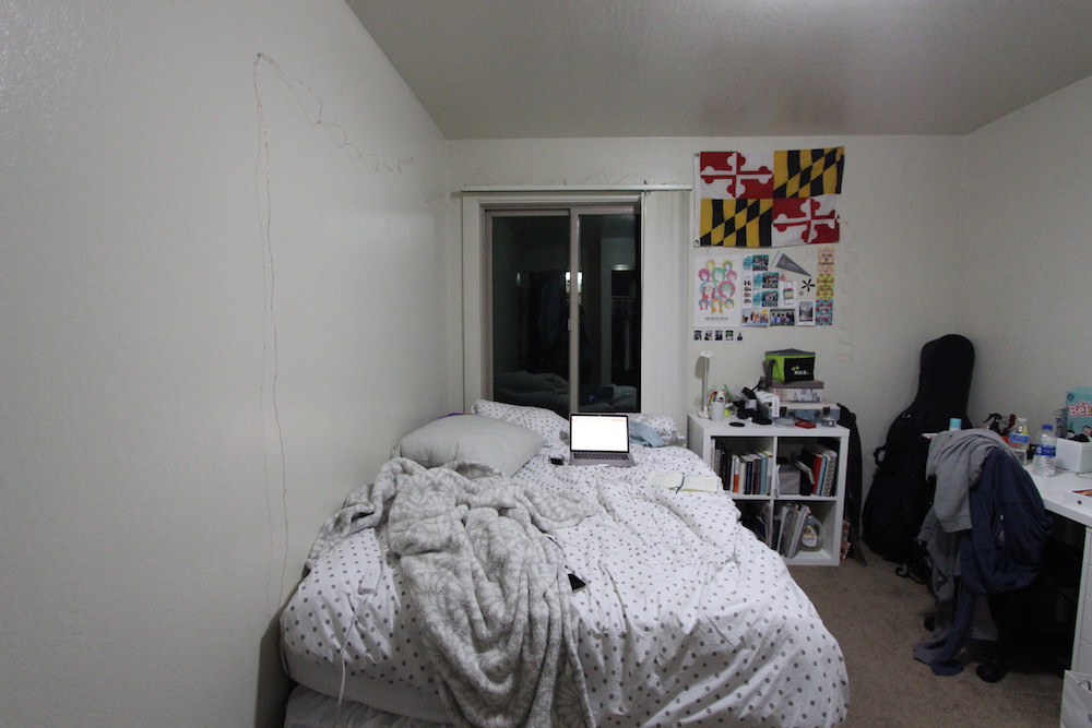
I took pictures of my room as well as my friends.
Part A2: Recover Homographies
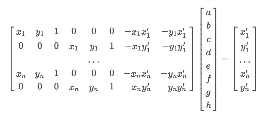
In order to warp our images, we need to find the correct transformation to apply to the points. The transformation is a
homography, meaning the relationship between the original points p and the target points p'
is represented by p' = Hp, where H is a 3x3 matrix of the form:
H matrix by finding the least-squares solution to the following overdetermined linear system:
Part A3: Rectify Images
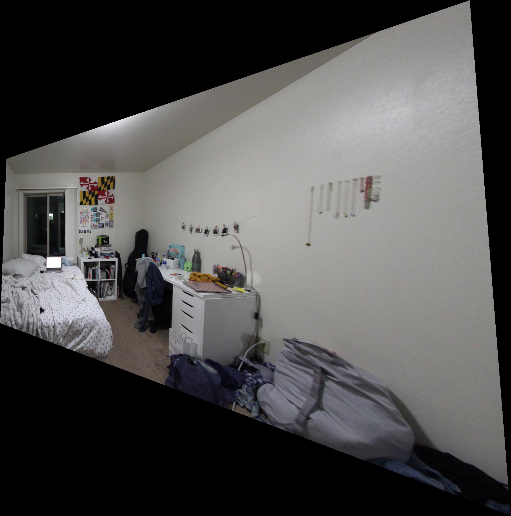
Now that we know how to find the correct transformation to warp our images, we can use this method to rectify our images –
or warp the image so some flat surface in the image can be made frontal-parallel. We do this by defining a set of 4 points
in the source image; defining the corners of some rectangular shape whose perspective makes it non-rectangular in the image.
Then we can define a rectangular shape to warp that section of the image to, in order to find H. Once we have the
correct matrix, we can use inverse warping and bilinear interpolation to map the pixels from the source image to the correct,
straightened output image.
| Original | Rectified |
|---|---|
|
|
|
|
|
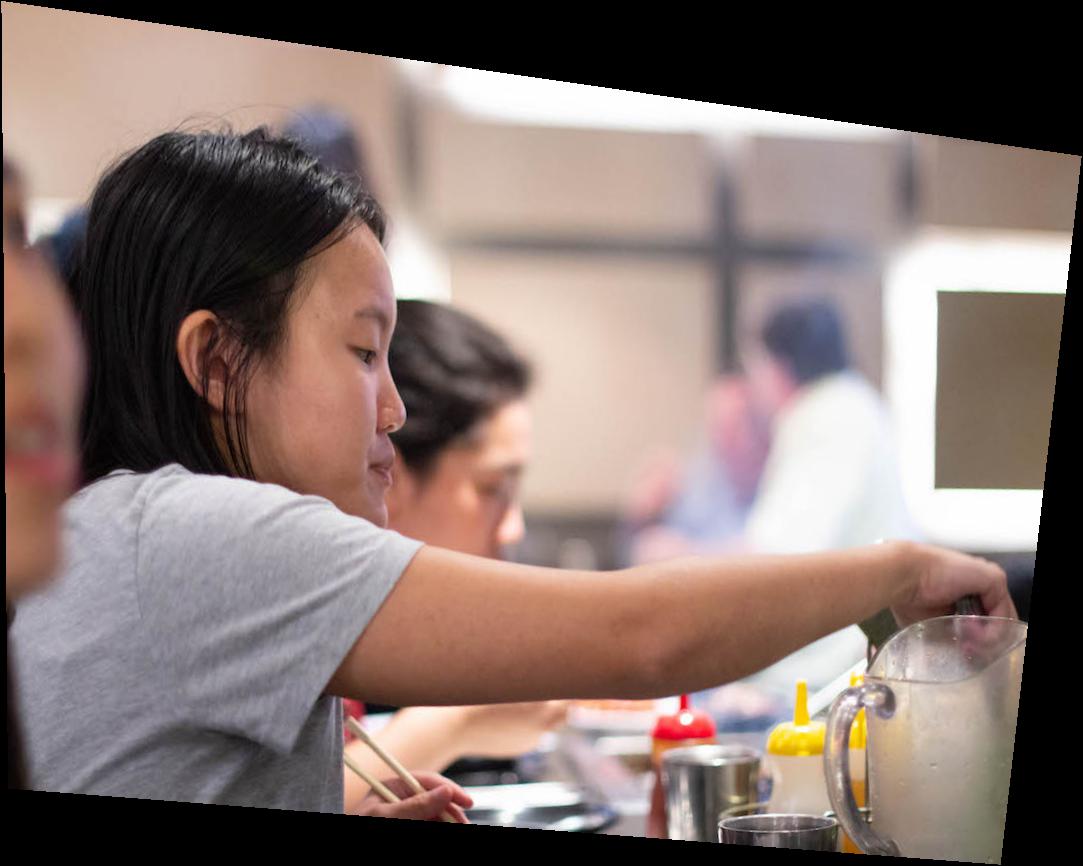
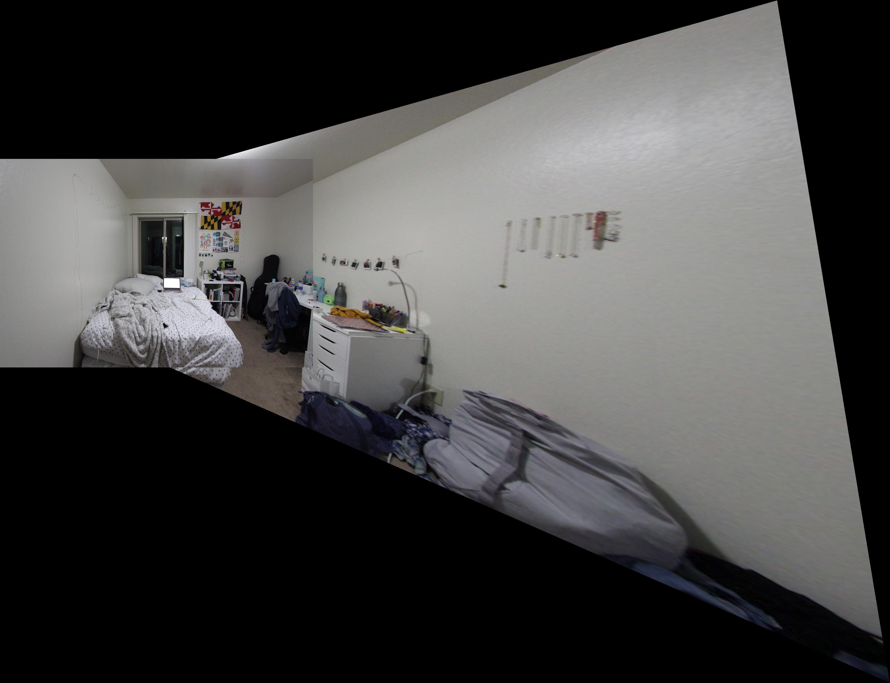
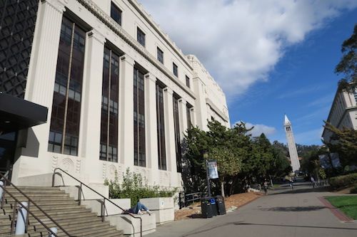
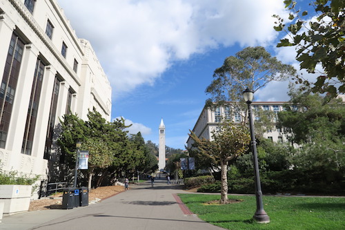
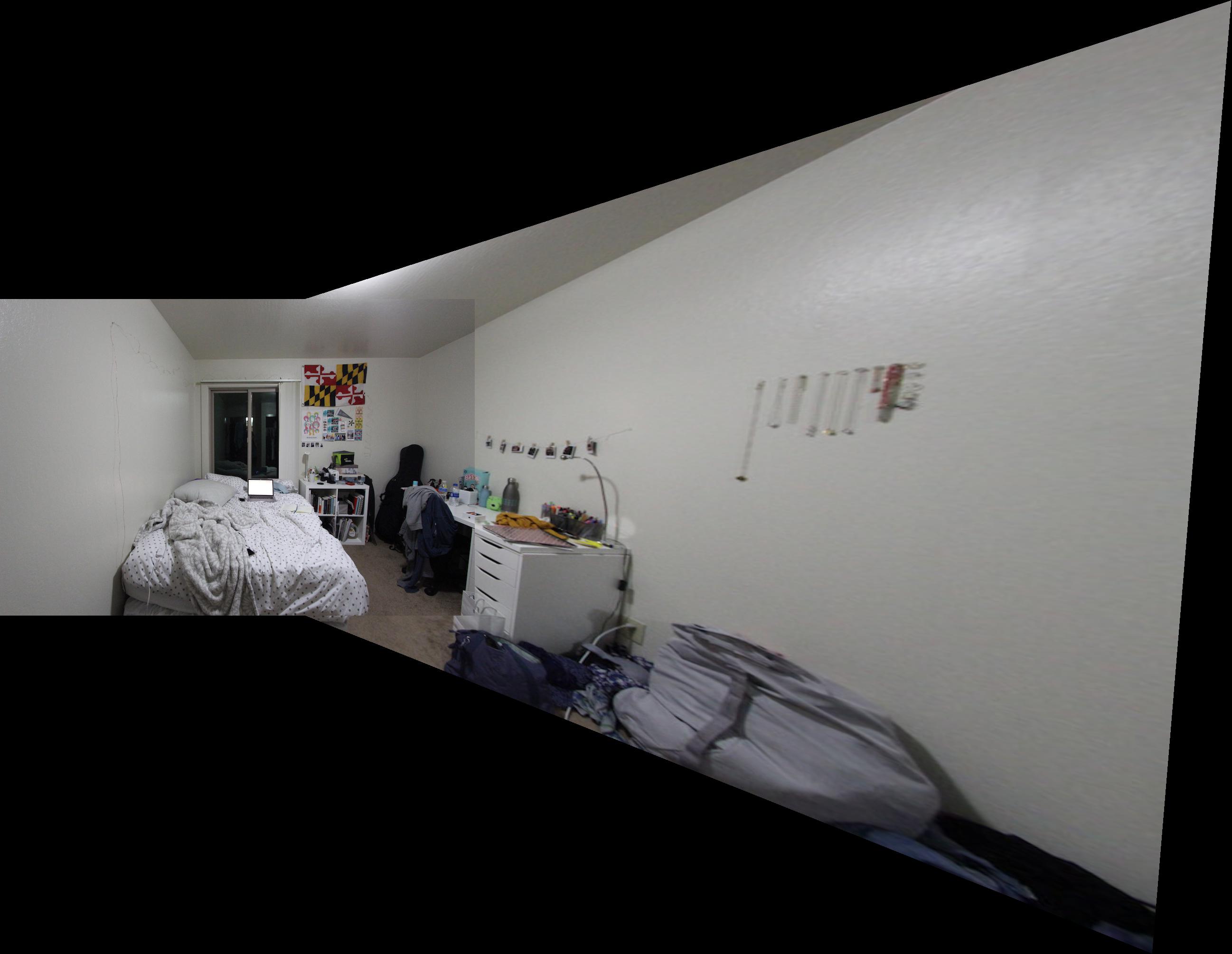
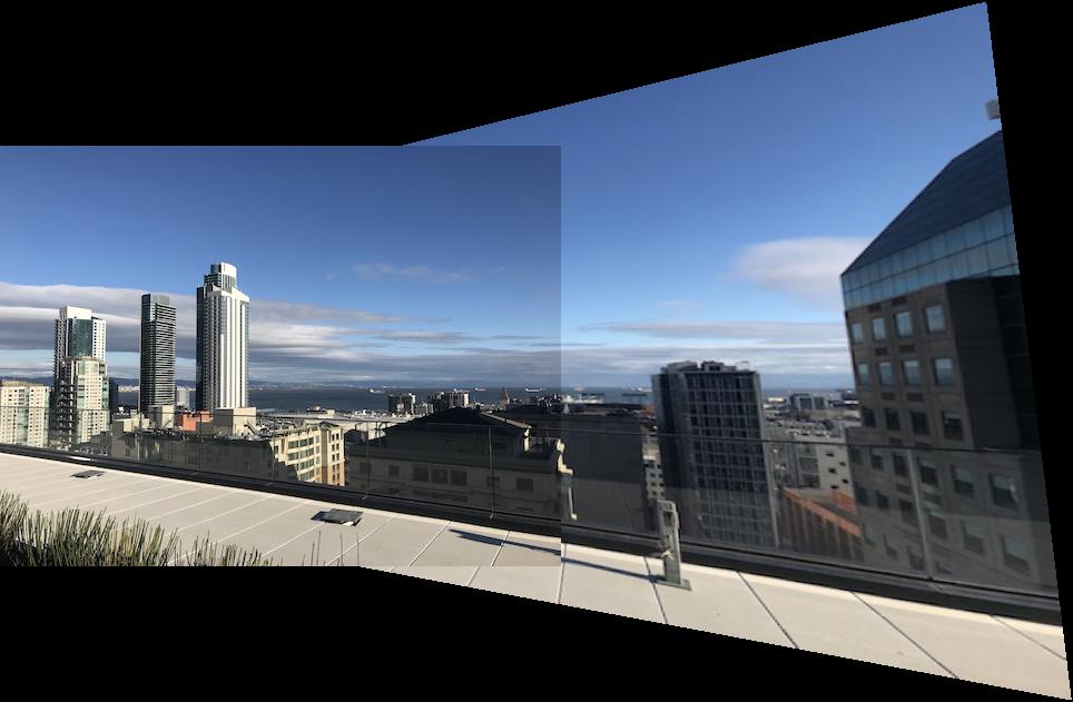
Part A4: Mosaic
Instead of simply warping one image to a rectangle, we can take two images of the same scene at slightly different perspectives and define correspondances that will allow us to warp one image to the shape of the other. Then, we can overlay them such that the correspondances are on top of each other, creating a photo mosaic.
| Left | Right | Mosaic |
|---|---|---|
|
|
|
|
Part B1: Harris Corners
While we were able to produce okay results by manually choosing correspondances, in this section we use techniques that will
allow us to automatically detect correspondances between two images in order to create our photo mosaics. We will be using
the methods described in this paper.
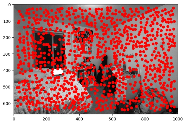
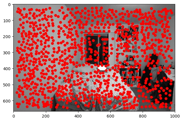
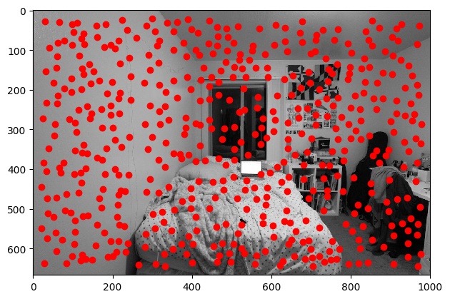
We first start with the Harris Interest Point Detector, which was provided for us by staff. I changed the min_distance
parameter from 1 to 10, because it originally gave way too many points such that essentially the
entire image was covered with Harris corners.
| Left | Right | |
|---|---|---|
| Original |
|
|
| Harris Corner |
|
|
Part B2: Adaptive Non-Maximal Suppression
While we limited some of the points by adjusting the min_distance parameter, we still have a lot of points,
which will lead to a lot of overhead when it comes to finding correspondances in the later parts of the project. Therefore,
we'd like to further limit our search by choosing the Harris points that have the greatest corner strength. However,
at the same time we don't want all of our resulting points to be clustered around the same area. In order to choose points
while satisfying both of these requirements, we use the Adaptive Non-Maximal Suppression (ANMS) algorithm, which calculates
a radius value r_i for each point as defined by the following equation, where x_i is the point
corresponding to the calculated r_i, x_j are all other points of interest, f is the
function mapping interest points to their Harris corner strength, and c_robust is a constant factor:
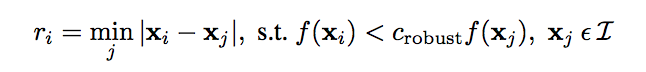
As specified in the paper, we use c_robust = .9 and chose the 500 points with the largest
r_i values.
| Left | Right | |
|---|---|---|
| Harris Corner |
|
|
| Post-ANMS |
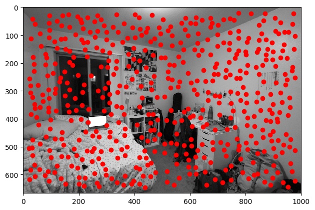
|
|
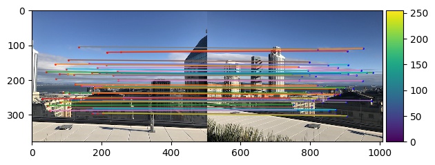
Part B3: Feature Descriptor Extraction and Feature Matching
Now that we have a good number of points to work with, we need to start figuring out how we're going to match corresponding points
between the two images. We first start by defining features around each interest point. For each interest point, we find
a 40x40 patch centered on the point of interest, apply a Gaussian blur to reduce noise, and then resize the patch
to 8x8. In order to find the corresponding feature patch between images, we find the closest matching patch pairs
between the two images by flattening each feature patch and calculating the Euclidean distance between the two. In order to ensure
that we are only keeping correspondances that we are very confident about, we only keep points whose first nearest neighbor is
significantly better matched than the second nearest neighbor. This is Lowe's technique and means we only choose
points that satisfy e_1nn / e_2nn < threshold , where e_1nn is the distance/error of the first nearest
neighbor and e_2nn is the distance/error of the second nearest neighbor, and threshold is a decimal
value between 0 and 1 that we decide. Here, I have used threshold = .1. The correspondance
code is provided by Ajay Ramesh.
| Left | Right | Correspondances |
|---|---|---|
|
|
|
|
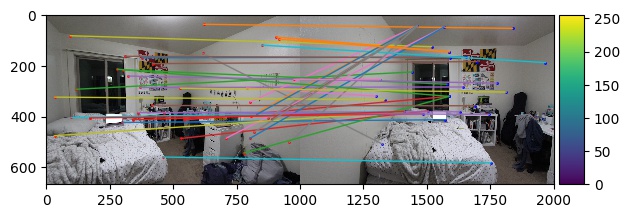
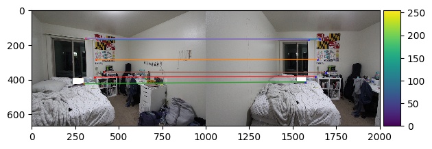
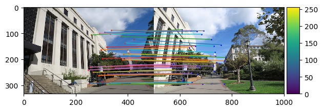
Part B4: Random Sample Consensus
With our potential correspondances, we will further narrow down our correspondances using Random Sample Consensus (RANSAC). In
this algorithm, we randomly select 4 points to produce a homography transformation H and find the corresponding
error by calculating the L2-norm between the transformed points and the input points and only keeping the points
whose error is less than a certain threshold. We then choose the homography transformation matrix that leads to the greatest number
of points preserved after eliminating those outside of our error bound as well as the corresponding points. These are the
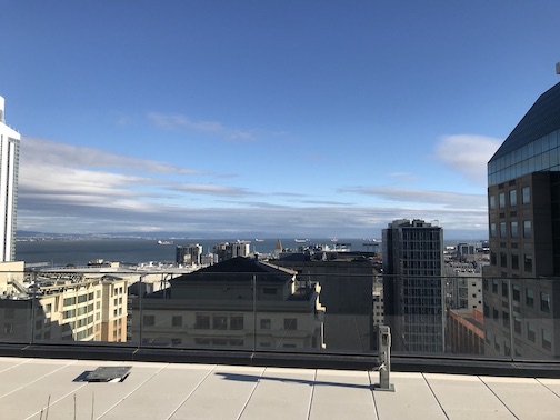
resulting correspondances. Some of the following images were found online as parts of previous assignments.
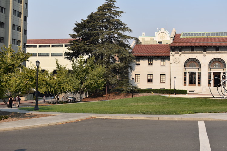
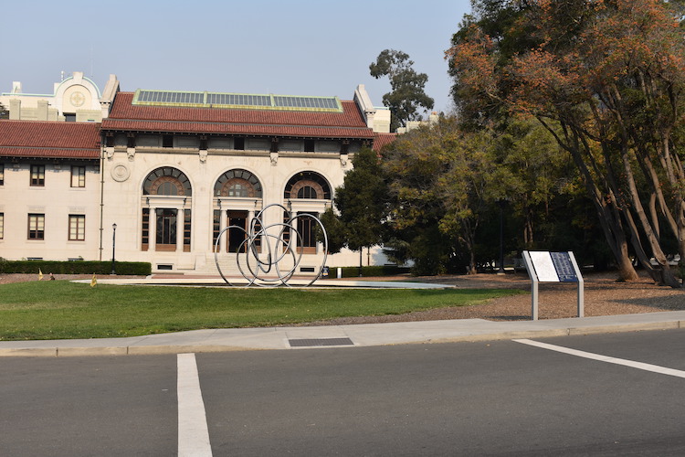
| Left | Right | Correspondances |
|---|---|---|
|
|
|
|
|
|
|
|
|
|
|
|
|
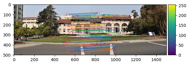
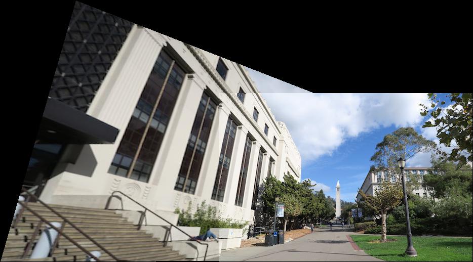
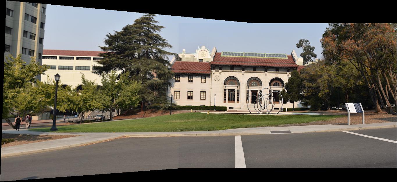
Part B5: AutoStitching
Now that we have correspondances, we can use the same mosaic algorithm that we used before with manually-defined correspondances. Here are some of the results.
| Left | Right | Correspondances |
|---|---|---|
|
|
|
|
|
|
|
|
|
|
|
|
|
|
|
|
What I Learned
I think the coolest thing I learned from this project was the Random Sample Consensus algorithm. It makes a lot of sense to sample many different homographies and choose the one that results in the most correct points, and it seems to work pretty well!